Units, Dimensions, and Significant Figures in Measurement
An introduction to physical quantities, units, systems of measurement, significant figures, and the handling of errors and uncertainty in scientific measurements.
In the study of physics, we do not merely observe the world; we quantify it. To describe the laws of nature, we rely on measurable properties known as physical quantities. Whether we are measuring the mass of a particle, the length of a beam, or the duration of an event, the accuracy and consistency of these measurements form the foundation of all scientific inquiry. This article explores how we define these quantities, the systems we use to standardize them, and the mathematical rules required to handle the inherent uncertainties in every measurement.
Physical Quantities and Units
A physical quantity is any property that can be measured. These quantities are the building blocks of physical laws, encompassing everything from temperature and pressure to electric current and resistance. To ensure that a measurement is meaningful, we must compare it to a reference standard known as a unit.
Classification of Quantities
Physical quantities are categorized into two distinct groups:
Fundamental Quantities: These are independent quantities that cannot be defined in terms of others. Examples include mass, length, and time.
Derived Quantities: These are quantities expressed as combinations of fundamental quantities. For example, velocity is derived from length and time.
For a unit to be scientifically valid, it must meet several strict criteria: it must be of a suitable size, well-defined, easily reproducible, and stable across different times, places, and physical conditions like temperature or pressure.
Systems of Measurement
Throughout history, different systems of units have been utilized. While various regional systems exist, modern science relies on standardized frameworks:
FPS System: Uses Foot, Pound, and Second.
CGS System: Uses Centimetre, Gram, and Second.
MKS System: Uses Metre, Kilogram, and Second.
SI System (International System): The global standard used in almost all scientific applications.
The SI system is built upon seven basic units: the metre (length), kilogram (mass), second (time), kelvin (temperature), ampere (electric current), mole (amount of substance), and candela (luminous intensity).
This diagram illustrates the relationship between fundamental SI units (mass, length, time) and derived units (speed, acceleration, force, density) through combination and mathematical operations.
Significant Figures and Precision
Every measurement contains a degree of uncertainty. When we record a value, we include all the digits we are certain of, plus one final digit that is uncertain. This total count of reliable and uncertain digits is known as significant figures. The number of significant figures reflects the precision of the instrument used; a more precise instrument will yield more significant figures.
Rules for Determining Significant Figures
To correctly identify significant figures, follow these rules:
All non-zero digits are always significant.
Zeros located between two non-zero digits are significant.
Leading zeros (those appearing before the first non-zero digit) are not significant.
Trailing zeros are significant only if a decimal point is present in the number.
To avoid ambiguity, especially when dealing with very large or very small numbers, scientists use scientific notation (a×10b). In this format, the power of 10 is considered irrelevant to the precision, so the number of significant figures is determined solely by the coefficient a.
Exam Tip: When multiplying or dividing exact numbers (like the "2" in the formula for radius), treat them as having an infinite number of significant figures so they do not limit the precision of your final result.
Arithmetic Operations
When performing calculations, you must follow specific rules to ensure your result does not claim more precision than your measurements allow:
Multiplication and Division: The final result must have the same number of significant figures as the measurement with the least number of significant figures.
Addition and Subtraction: The final result must have the same number of decimal places as the measurement with the least number of decimal places.
Example: Density Calculation
If Mass = 4.237 g (4 sig figs) and Volume = 2.51 cm3 (3 sig figs):
Density=VolumeMass=2.514.237=1.68804...=1.69 g/cm3
The result is rounded to 3 significant figures to match the volume.
Rounding Off Rules
When you need to reduce the number of digits, use these standard rounding procedures:
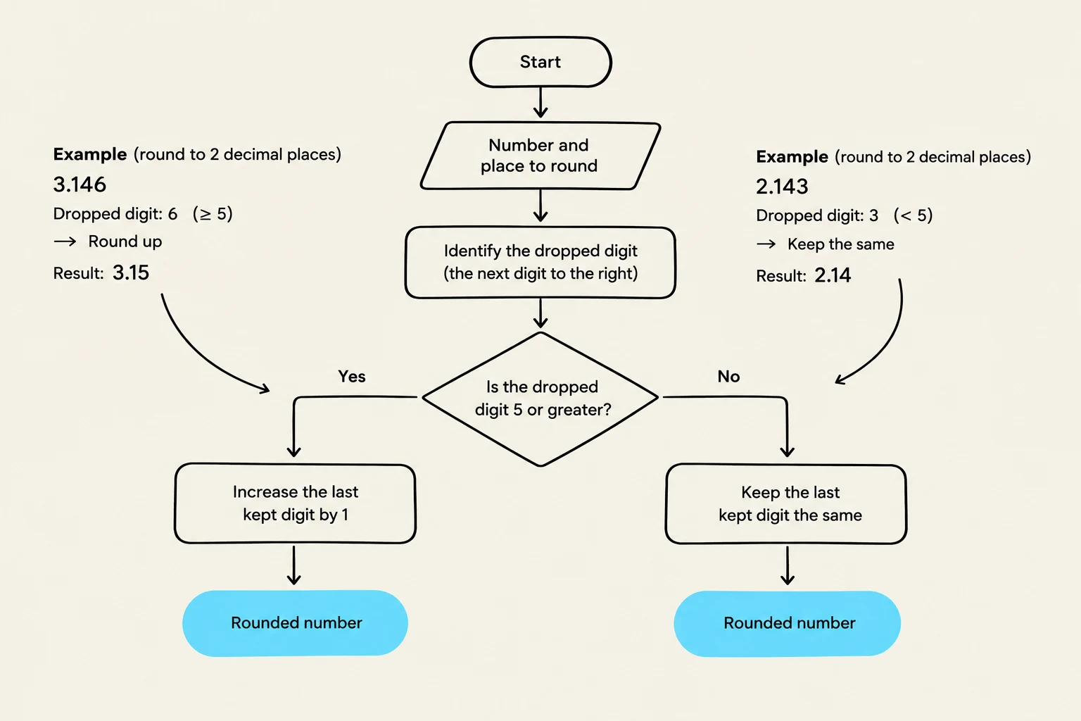
If the dropped digit is >5, increase the preceding digit by 1.
If the dropped digit is <5, leave the preceding digit unchanged.
If the dropped digit is exactly 5:
If the preceding digit is odd, increase it by 1.
If the preceding digit is even, leave it unchanged.
This flowchart illustrates the process of rounding numbers to a specified decimal place. It begins by identifying the number and the place to round to. Then, it examines the digit immediately to the right of the rounding place. If this digit is 5 or greater, the last kept digit is increased by 1. If the digit is less than 5, the last kept digit remains the same. The process concludes with a rounded number.
Errors and Uncertainty in Measurement
No measurement is perfect. The difference between a measured value and the true value is known as error. Understanding the source of these errors is vital for improving experimental accuracy.
Types of Errors
Errors can be classified based on their cause and behavior:
Least Count Error: This arises from the resolution limits of the instrument. The maximum possible error is often equal to the smallest scale division (the least count) of the device.
Instrumental Error: Caused by faulty calibration, such as a scale that does not read zero when nothing is on it (zero error), or physical changes like thermal expansion.
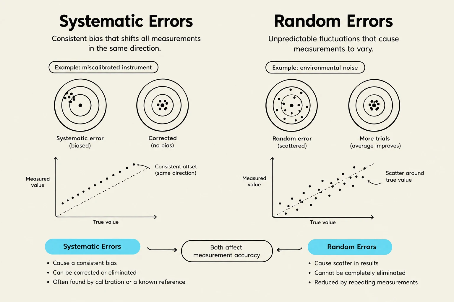
Random Error: These are unpredictable fluctuations that cause measurements to vary even when the same conditions are repeated. These errors typically follow a Gaussian (normal) distribution.
Accidental Error: These are unpredictable, extreme results (either much too high or much too low) that are usually excluded from final calculations.
Systematic Error: Errors that tend to deviate in a single direction (always positive or always negative), such as air buoyancy or imperfect experimental techniques.
Calculating Uncertainty
Uncertainty can be quantified during arithmetic operations. For example, if a length is 16.2±0.1 cm, the ±0.1 represents the uncertainty. When performing multi-step computations, it is a best practice to keep one extra significant figure in intermediate steps to prevent the accumulation of rounding errors.
This illustration explains the concepts of systematic and random errors in measurements, providing examples and visual representations of each.
Summary Note: While errors are inevitable, understanding whether they are systematic or random allows scientists to apply corrections or use statistical methods to find the most probable true value.
Keep reading for free.
Create an account to finish this reading and make it part of your study routine.