Understanding the Risk-Return Tradeoff and Portfolio Diversification

Covariance and Correlation

Covariance ($\sigma_{i, j}$) measures the degree to which two assets move together.

• If $\sigma_{i, j} > 0$, the assets tend to move in the same direction.
• If $\sigma_{i, j} < 0$, the assets tend to move in opposite directions, which can help offset losses.

Because covariance can be difficult to interpret due to its scale, we use Correlation ($\rho_{i, j}$) to standardize the relationship. Correlation is a scaled version of covariance that always falls between $-1$ and $1$:

$\rho_{i, j}=\frac{\sigma_{i, j}}{\sigma_{i} \sigma_{j}}$

• $\rho = 1$ (Perfect Positive): The assets move in perfect lockstep.
• $\rho = 0$ (No Correlation): There is no linear relationship between the assets.
• $\rho = -1$ (Perfect Negative): The assets move in exactly opposite directions.

Portfolio Theory: Return and Risk

A portfolio is a collection of assets, each weighted by the proportion of total wealth invested in it ($X_i$).

Portfolio Expected Return

The expected return of a portfolio ($E(R_p)$) is simply the weighted average of the expected returns of the individual assets:

$E(R_{p}) = \sum_{i=1}^{N} X_{i} R_{i}$

Portfolio Variance and Risk

Unlike return, Portfolio Variance ($\sigma_p^2$) is not a simple weighted average of individual variances. It must account for the way assets covary. For a two-asset portfolio, the formula is:

$\sigma_{p}^{2} = X_{1}^{2} \sigma_{1}^{2}+X_{2}^{2} \sigma_{2}^{2}+2 X_{1} X_{2} \rho_{1,2} \sigma_{1} \sigma_{2}$

The final Portfolio Risk is the standard deviation of this variance: $\sigma_{p}=\sqrt{\sigma_{p}^{2}}$.

The Power of Diversification

Diversification is the process of reducing risk by investing in assets that do not move perfectly together. The effectiveness of this strategy depends entirely on the correlation ($\rho$) between assets.

Figure: Risk Return Trade-off: Portfolios of N=2 Assets

As shown in the figure above, different correlations create different "frontiers" of possible outcomes:

• Perfect Positive Correlation ($\rho = 1$): The frontier is a straight line. No risk reduction is achieved through diversification.
• No Correlation ($\rho = 0$): The frontier curves toward the left, indicating that risk can be reduced for a given level of return.
• Perfect Negative Correlation ($\rho = -1$): The frontier reaches all the way to the vertical axis. In this theoretical scenario, it is possible to construct a Minimum Variance Portfolio with zero risk.

Diversifying Across Many Assets

What happens if we move beyond two assets? If we invest equally in $N$ stocks, the portfolio variance can be expressed as:

$\sigma_{p}^{2}=\frac{1}{N} \bar{\sigma}_{i}^{2}+\frac{N-1}{N} \bar{\sigma}_{i, k}$

As the number of assets $N$ approaches infinity ($N \rightarrow \infty$), the first term (representing individual security risk) approaches zero. This means that idiosyncratic risk (risk specific to a single company) can be diversified away, leaving only systemic market risk.

The Efficient Frontier and Investor Preferences

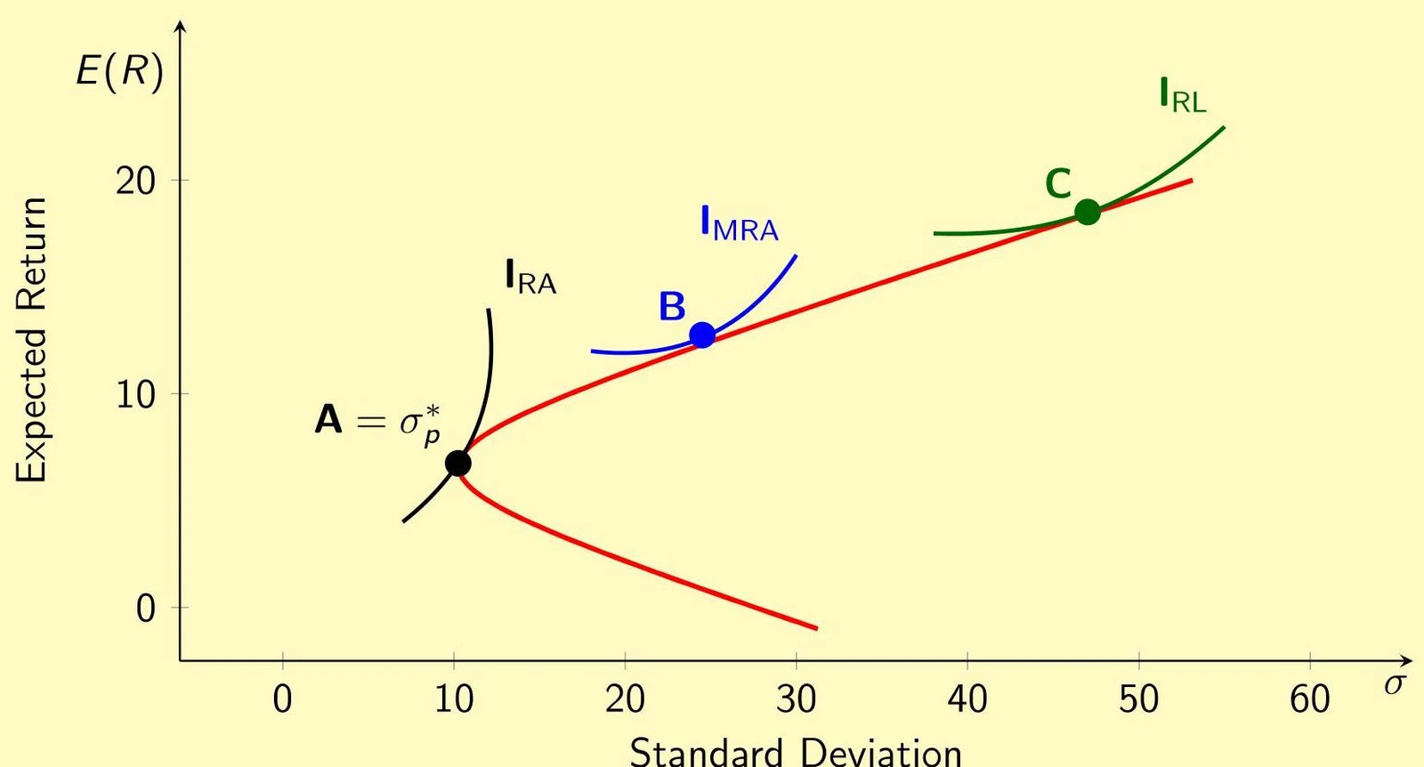
When we plot all possible combinations of assets on a graph of Expected Return vs. Standard Deviation, we create the Mean-Standard Deviation Frontier.

Efficient vs. Inefficient Portfolios

• Efficient Portfolios: These lie on the upper segment of the frontier. They represent the maximum possible return for a given level of risk.
• Inefficient Portfolios: These lie on the lower segment. An investor would never choose these because they could achieve a higher return for the same amount of risk by moving to the upper segment.

Individual Risk Aversion

While the Efficient Frontier tells us what is possible, an investor's personal preferences tell us what is optimal. We use indifference curves to represent these preferences. An indifference curve connects points that provide the same level of "utility" or happiness to an investor.

The slope of these curves represents an investor's risk aversion:

• High Risk Aversion: Very steep curves. These investors require a massive increase in expected return to accept even a small increase in risk.
• Low Risk Aversion: Flatter curves. These investors are willing to accept more risk for relatively small increments in return.

The optimal portfolio for any specific investor is found at the point where their highest possible indifference curve is tangential to the efficient frontier.