When you invest money, you are often looking at a single number: the interest rate offered by a bank or a bond. However, that number doesn't tell the whole story. To understand whether your wealth is actually growing, you must distinguish between the number you see on your statement and the actual increase in your ability to buy goods and services. This distinction is the foundation of the Fisher equation.
Understanding the Three Pillars of Interest Rates
To master the relationship between inflation and returns, we must define three distinct concepts: the nominal interest rate, the real rate of interest, and expected inflation.
1. The Nominal Interest Rate (rnom)
The nominal interest rate is the "advertised" rate. It is the percentage increase in the amount of money you have at the end of a period. For example, if you invest $100 at a 5% nominal interest rate, you will have $105 at the end of the year. While this looks like growth, it does not account for the fact that prices in the economy might have also risen during that time.
2. Expected Inflation (E(i))
Inflation is the rate at which the general level of prices for goods and services rises, subsequently eroding purchasing power. In financial modeling, we specifically look at expected inflation—what market participants believe the inflation rate will be over their investment horizon.
3. The Real Rate of Interest (rreal)
The real rate of interest is the most critical metric for an investor. It represents the actual growth in your purchasing power. If your money grows by 5% (nominal), but the cost of living grows by 3% (inflation), your real rate of interest is approximately 2%.
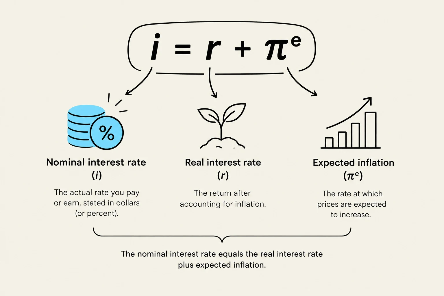
This diagram illustrates the relationship between nominal interest rate, real interest rate, and expected inflation, represented by the formula i = r + πe.
The Fisher Equation
The relationship between these three components is expressed through the Fisher equation:
rnom=rreal+E(i)
This equation tells us that the nominal interest rate is essentially a compensation for two things: the desire to grow real wealth (rreal) and the need to offset the loss of purchasing power caused by inflation (E(i)).
Worked Example
Suppose the real rate of interest is 2%, and expected inflation is 4%. Using the Fisher equation:
rnom=2%+4%=6%
If market expectations change and expected inflation rises to 5%, the nominal interest rate should climb to 7% to maintain that same 2% rate of purchasing power.
Concept Check
Question a: Suppose the real interest rate is 3% per year and the expected inflation rate is 8%. What is the nominal interest rate?
Question b: Suppose the expected inflation rate rises to 10%, but the real rate is unchanged. What must happen to the nominal interest rate?
(Answers: a. 11%; b. The nominal rate must rise to 13%)
Empirical Evidence: Treasury Bills and Inflation
To see how this works in the real world, economists often look at Treasury bills (T-bills). Because T-bills are backed by the government, they provide a clear look at how nominal rates respond to inflation over long periods.
Historical data from 1927 to 2022 shows how these variables shift over time. For instance, in the period from 1927 to 1951, the average nominal rate on T-bills was quite low at 0.95%, while inflation averaged 1.80%. This resulted in a negative average real rate of -0.48%.
In contrast, the post-war period (1952–2022) saw higher nominal rates (4.11%) and higher inflation (3.50%), which allowed for a positive average real rate of 0.61%.
Table 5.2: Statistics for T-bill rates, inflation rates, and real rates, 1927–2022
Category
Average Annual Rates: T-Bills
Average Annual Rates: Inflation
Average Annual Rates: Real T-Bill
Standard Deviation: T-Bills
Standard Deviation: Inflation
Standard Deviation: Real T-Bill
Full sample
3.28
3.06
0.32
3.09
3.97
3.80
1927–1951
0.95
1.80
-0.48
1.24
6.06
6.34
1952–2022
4.11
3.50
0.61
3.13
2.85
2.34
Note: The real rate in each year is computed as (1+rnom)/(1+i)−1.
This graphic illustrates the difference in volatility between inflation and real interest rates during two distinct periods: 1927-1951, characterized by high volatility, and 1952, which exhibited much more stable rates.
The Role of Volatility and Predictability
One of the most important takeaways from historical data is the importance of the standard deviation of real rates. The standard deviation measures how much a value fluctuates around its average.
If you look at Table 5.2, there is a dramatic difference in the stability of real returns between the two time periods:
1927–1951: The standard deviation of the real rate was 6.34%.
1952–2022: The standard deviation of the real rate dropped to 2.34%.
Why did this happen? The data suggests that after 1952, inflation became far less volatile. When inflation is more predictable, the nominal interest rate can track it much more reliably.
Key Insight
The Fisher relation works most effectively when inflation is predictable. When inflation is stable, investors can more accurately gauge the nominal interest rate required to achieve an acceptable real rate of return.
This diagram illustrates the relationship between stable inflation, nominal interest rates, and real interest rates, showing that stable inflation leads to more predictable nominal rates and more stable real rates.
In summary, while the nominal rate is what you see, the real rate is what you feel. The Fisher equation serves as the bridge between the two, helping investors navigate the complexities of inflation and purchasing power.
Keep reading for free.
Create an account to finish this reading and make it part of your study routine.