Understanding the Describing Function Method in Control Systems
This guide explains the describing function method, a technique used in control systems engineering to analyze nonlinear elements by approximating their behavior with harmonic linearization. It covers the core concepts, mathematical derivations, and provides examples for relay, deadzone, and saturation nonlinearities.
In control systems engineering, analyzing nonlinear elements can be significantly more complex than analyzing linear ones. While linear systems can be solved using standard transfer functions, nonlinearities often produce outputs that are not simple scaled versions of their inputs. To bridge this gap, engineers use the describing function method, a technique based on harmonic linearization. This method approximates the effect of a nonlinearity by focusing on how it transforms a sinusoidal input into a fundamental sinusoidal output component.
The Core Concept: Harmonic Linearization
The describing function method assumes that if a nonlinear element is part of a system with low-pass characteristics (such as a plant with significant inertia or capacitance), the higher-order harmonics produced by the nonlinearity will be filtered out. Consequently, the input to the nonlinearity remains a pure sinusoidal signal, and the analysis can focus solely on the fundamental component of the output.
Consider a nonlinear element N with an input x(t)=Xsin(ωt). The resulting output y(t) is generally a non-sinusoidal periodic function. To analyze this, we represent y(t) using a Fourier series:
The describing function, denoted as N(X,ω), is defined as the ratio of the fundamental output amplitude (γ1) to the input amplitude (X), assuming the phase shift (ϕ1) is zero:
N(X,ω)=Xγ1∠ϕ1
To find the fundamental amplitude γ1 and phase ϕ1, we use Fourier coefficients calculated via definite integrals:
A1=π2∫0πysin(ωt)d(ωt)B1=π2∫0πycos(ωt)d(ωt)
Where the amplitude is γ1=A12+B12 and the phase is ϕ1=tan−1(A1B1).
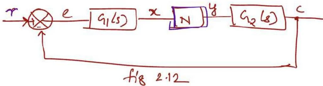
A block diagram illustrating a control system with components G1(s), N, and G2(s), and signals r, e, x, y, and c.
Exam Tip: When performing these derivations, always check if the nonlinearity is symmetric. If the nonlinearity is an odd function (like a relay or deadzone), the output will have no even harmonics and no DC component (A0=0), and the phase shift ϕ1 will typically be zero.
1. Relay (On-Off) Nonlinearity
A relay nonlinearity is a switching element that jumps between two fixed values, +m and −m. This is commonly seen in thermostat controls or simple bang-bang controllers.
When a sinusoidal input x(t)=Xsin(ωt) is applied, the output y(t) switches between m and −m at the points where the input crosses zero. To find the describing function, we calculate the fundamental Fourier coefficient A1 using the integral:
A1=π2∫0πysin(ωt)d(ωt)
For a relay switching between ±m, the integration yields a fundamental amplitude of Y1=π4m. Therefore, the describing function for a relay is:
N(X,ω)=πX4m
Note that the gain of a relay decreases as the input amplitude X increases, because the "switching" happens less frequently relative to the period of the sine wave.
2. Deadzone Nonlinearity
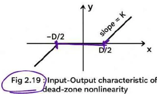
A deadzone nonlinearity is characterized by a region where the input produces zero output. This occurs when the input magnitude is less than a threshold, often denoted as D/2. Once the input exceeds this threshold, the output follows a linear relationship with slope k.
A graph illustrating the input-output characteristic of a dead-zone nonlinearity, showing a region where the output is zero for a range of inputs, and linear behavior outside this range.
To derive the describing function, we must integrate the output only over the intervals where the input is outside the deadzone. Let α be the angle where the input reaches the deadzone threshold, such that sin(α)=2XD.
After solving the definite integrals for the linear segments, the describing function is found to be:
N(X,ω)=k1−π2sin−1(2XD)+2XD1−(2XD)2
This formula shows that as X becomes very large compared to D, the term in the brackets approaches 1, and the nonlinearity behaves like a pure linear gain k. However, as X approaches D/2, the effective gain drops to zero.
3. Saturation Nonlinearity
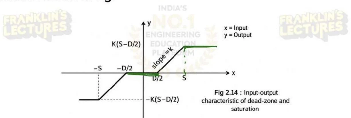
Saturation occurs when a system's output increases linearly with the input up to a certain limit S, but then remains constant (saturates) regardless of further increases in the input.
Input-output characteristic of dead-zone and saturation.
In this case, the output y(t) is kx(t) when ∣x(t)∣<S, and y(t)=±kS when ∣x(t)∣≥S. To find the describing function, we define β as the angle where the input reaches the saturation limit, such that sin(β)=XS.
The fundamental amplitude Y1 is calculated by integrating the linear part and the saturated part separately:
Solving these integrals leads to the describing function:
N(X,ω)=π2ksin−1(XS)+XS1−(XS)2
As the input amplitude X increases, the ratio S/X decreases, causing the effective gain of the describing function to decrease. This reflects the fact that a larger portion of the input signal is spent in the "saturated" region where the gain is effectively zero.
By replacing the complex nonlinear block with its corresponding describing function N(X,ω), engineers can use frequency-domain techniques like Nyquist or Bode plots to analyze the stability and limit cycle behavior of nonlinear control systems.
Keep reading for free.
Create an account to finish this reading and make it part of your study routine.