This content explains how taxes affect markets, distinguishing between statutory and economic burdens, and demonstrating how price elasticity determines who ultimately bears the cost of a tax.
When governments intervene in a market, they often do so by imposing taxes to raise revenue or to discourage certain behaviors, such as the consumption of sugary drinks. While it might seem intuitive that the party responsible for sending the tax check to the government bears the full cost, economic reality is far more complex. To understand how a tax truly affects a market, we must distinguish between who is legally responsible for the tax and who actually feels the financial sting.
Statutory vs. Economic Burden
To analyze taxes effectively, we must first define two critical terms: statutory burden and economic burden.
Statutory Burden: This is the legal obligation assigned by the government. If a law states that a shopkeeper must collect and remit a tax on every soda sold, the statutory burden lies with the seller.
Economic Burden: This refers to the actual change in the after-tax prices faced by buyers and sellers.
The most important takeaway for any student of economics is that the tax incidence—the division of the economic burden—does not depend on the statutory burden. Whether the government collects the tax from the buyer at the register or from the seller at the end of the month, the final impact on the market equilibrium is identical.
Assessing a Tax on Sellers
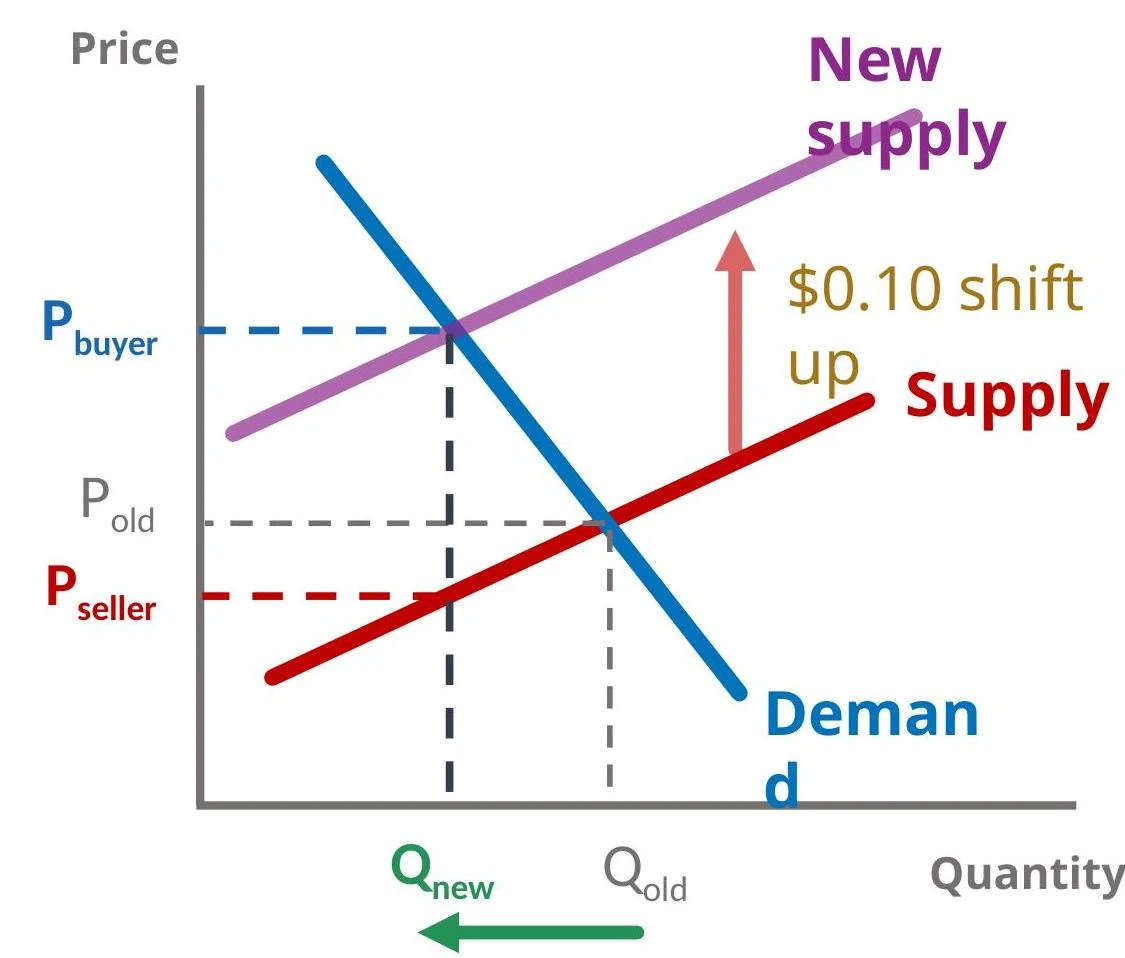
When a tax is imposed on sellers, it is viewed as an increase in their marginal costs of production. Because the supply curve represents the marginal cost curve, a tax on sellers causes the supply curve to shift "upward" (or to the left) by the exact amount of the tax.
This graph illustrates the economic concept of supply and demand, showing how a shift in supply affects the equilibrium price and quantity of soda.
Consider a soda tax of $0.30 per unit. When the supply curve shifts up, a new equilibrium is formed where the new supply curve intersects the original demand curve. This results in two different prices:
The Price Buyers Pay: This is typically higher than the original equilibrium price.
The Price Sellers Receive: This is the price buyers pay minus the tax amount sent to the government.
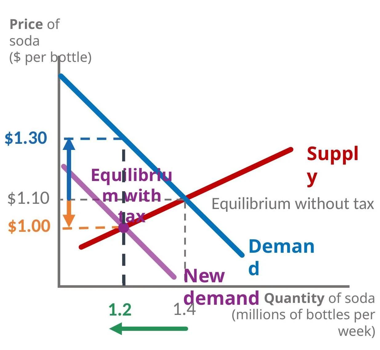
This graph illustrates the economic impact of a tax on soda. The demand curve slopes downward, while the supply curve slopes upward. The initial equilibrium without tax is at a price of $1.10 and a quantity of 1.4 million bottles per week. After a tax is imposed, the supply curve shifts upward, leading to a new equilibrium with a higher price of $1.30 and a lower quantity of 1.2 million bottles per week.
The difference between these two prices represents the tax collected by the government.
Assessing a Tax on Buyers
If the government instead imposes the tax on buyers, the mechanism of the shift changes, but the outcome remains the same. A tax on buyers reduces the marginal benefits of consuming the good. Since the demand curve represents the marginal benefit curve, the tax causes the demand curve to shift "downward" (or to the left) by the amount of the tax.
This graph illustrates the economic concept of demand and supply, showing how a shift in demand affects the equilibrium price and quantity of soda.
The new equilibrium is found where this new demand curve intersects the original supply curve. Just as in the previous scenario, the quantity sold decreases, and a "wedge" is created between what the buyer pays and what the seller receives.
This graph illustrates the economic impact of a tax on soda. It shows the original demand and supply curves, the equilibrium point without tax, and how a new demand curve and equilibrium are established after a tax is imposed, leading to a higher price and lower quantity.
The Role of Elasticity in Tax Incidence
If the market outcomes are identical regardless of who is taxed, how do we determine how much of the burden falls on the buyer versus the seller? The answer lies in price elasticity.
Tax incidence is determined by the relative elasticities of the supply and demand curves. A fundamental rule of thumb is: the more inelastic party bears more of the tax burden.
Inelastic Demand: If buyers are relatively unresponsive to price changes (a steeper demand curve), they will pay a larger share of the tax.
Elastic Demand: If buyers are very responsive to price changes (a flatter demand curve), they will pay a smaller share, and the sellers will absorb more of the cost.
Summary of Elasticity Impacts
Scenario
Relative Elasticity
Who bears more burden?
Demand is more inelastic than Supply
Buyers are less responsive
Buyers
Supply is more inelastic than Demand
Sellers are less responsive
Sellers
Exam Tip: The Four-Step Recipe for Evaluating Taxes
Identify the shift: Which curve is shifting (supply or demand)?
Direction of shift: Is it an increase or decrease? (Taxes shift curves to the left/down).
Compare equilibriums: Find the new price for buyers and the new price for sellers.
Determine incidence: Compare the elasticities. The more inelastic party pays more.
Worked Example: The Gas Tax
Imagine Louisiana considers a new tax of $0.10 per gallon of gas, with the statutory burden placed on sellers.
Which curve shifts? The supply curve shifts because the tax is an increase in marginal cost.
Direction? The supply curve shifts up and to the left.
Outcomes? The quantity of gas sold will decrease. The price buyers pay will rise, and the price sellers receive will fall.
Incidence? Looking at the provided graph, the demand curve is steeper (more inelastic) than the supply curve. Therefore, buyers will bear the majority of the economic burden.
This graph illustrates the economic concept of supply and demand, showing how a shift in the supply curve affects equilibrium price and quantity.
Keep reading for free.
Create an account to finish this reading and make it part of your study routine.