Understanding Statistical Thinking and Research Methodology
A comprehensive guide to the principles of statistical thinking and research methodology, covering the basic investigation cycle, reliability, validity, p-values, confidence intervals, and the crucial distinction between correlation and causation.
Whether you are studying psychology, biology, or social sciences, the ability to think statistically is what separates casual observation from scientific inquiry. Scientific research is not merely about collecting facts; it is a systematic method of acquiring knowledge through measurement, testing, and evidence. To master this, one must understand how to move from a single observation to a broad conclusion, and how to distinguish between what is merely "related" and what actually "causes" an effect.
The Basic Investigation Cycle
Statistical thinking is not a linear path but a continuous cycle designed to minimize error and maximize understanding. This cycle typically follows four distinct stages:
Planning: The researcher defines the specific question they want to answer and determines what kind of data is required to address it.
Examining: Once data is collected, the researcher looks for patterns, examines distributions, and checks for data quality to ensure the information is reliable.
Inferring: This is the core of statistical thinking. Researchers use data from a small sample to make reasoned guesses about a much larger population.
Concluding: The researcher answers the original question while explicitly acknowledging the uncertainty and limitations of the findings.
Exam Tip: Induction vs. Deduction
Remember that Induction moves from specific observations to a general conclusion (e.g., "I saw three white swans, so all swans are white"), while Deduction moves from a general principle to a specific prediction (e.g., "All humans are mortal; Socrates is human; therefore, Socrates is mortal").
Reliability and Validity: Consistency vs. Accuracy
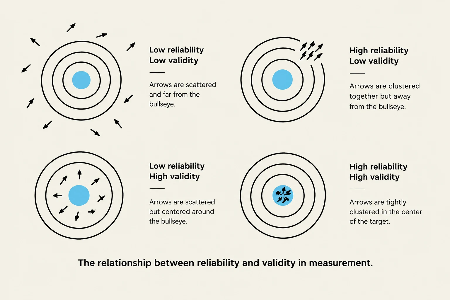
The relationship between reliability and validity in measurement is illustrated using target diagrams. These diagrams show four scenarios: low reliability and low validity (scattered and far from the bullseye), high reliability and low validity (clustered but away from the bullseye), low reliability and high validity (scattered but centered around the bullseye), and high reliability and high validity (tightly clustered in the center).
Before interpreting any result, you must evaluate the quality of the measurement tools used. A study can be consistent without being correct, or it can be accurate but impossible to replicate.
Reliability refers to consistency. A reliable measure is one that yields similar results under similar conditions. If a scale gives you a different weight every time you step on it within five minutes, it is not reliable.
Validity refers to accuracy. A valid measure actually captures the specific construct it intends to measure. For example, a math test that uses overly complex vocabulary might actually be measuring reading comprehension rather than math skills; in this case, the test lacks validity for math.
Interpreting Results: P-values and Confidence Intervals
When researchers analyze data, they use specific metrics to communicate how much confidence they have in their findings.
The Null Hypothesis and P-values
Most statistical tests begin with the null hypothesis, which is the assumption that there is no real effect or relationship in the population. The p-value is a summary of how "surprising" the observed data would be if the null hypothesis were actually true.
A small p-value (often p<.05) suggests that the data is very incompatible with the null hypothesis, providing evidence that an effect might exist. However, a p-value does not measure the probability that a hypothesis is true, nor does it measure the practical importance of the result.
Confidence Intervals and Uncertainty
Because we rarely study an entire population, our estimates are always slightly uncertain. A confidence interval provides a range of plausible values for a population parameter (the true value in the whole population) based on our sample data. The width of this range is determined by the margin of error, which reflects the level of uncertainty around the estimate.
Effect Size vs. Statistical Significance
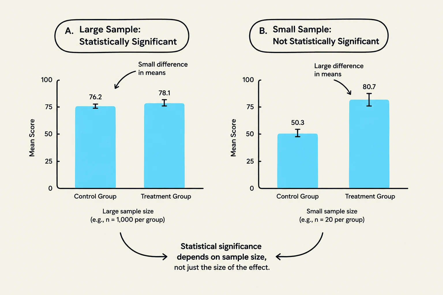
This illustration demonstrates how sample size affects statistical significance. A small difference in means can be statistically significant with a large sample size (A), while a large difference in means may not be statistically significant with a small sample size (B).
A common mistake is to assume that a "statistically significant" result is a "large" or "important" result. This is not necessarily true.
Statistical Significance asks: "Is this result unlikely to have happened by chance under the null model?".
Effect Size asks: "How large or meaningful is this relationship in the real world?".
Large samples can make even a tiny, practically useless difference appear "statistically significant". Conversely, a small sample might fail to reach statistical significance even if the effect is massive and practically important.
Methodological Rigor: Sampling and Assignment
To ensure a study is robust, researchers must be careful about how they select participants and how they organize them. There is a critical distinction between random sampling and random assignment.
Process
Question Answered
Primary Goal
Random Sampling
Who gets into the study?
Generalization: Ensuring the sample represents the population.
Random Assignment
Which condition do they enter?
Causal Conclusions: Balancing groups to isolate cause and effect.
The Golden Rule of ResearchRandom Sampling → Generalization (Can I apply this to everyone?)
Random Assignment → Causation (Did X cause Y?)
Correlation vs. Causation
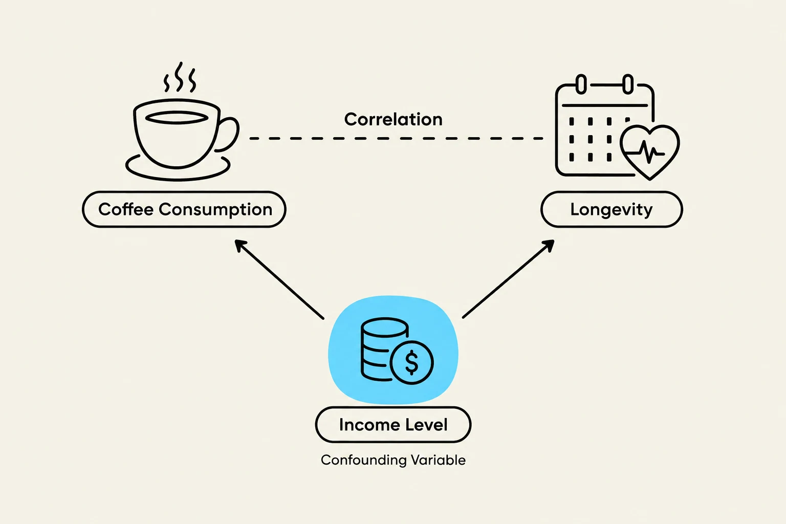
This diagram illustrates how income level can be a confounding variable in the correlation between coffee consumption and longevity.
One of the most fundamental rules in science is that correlation/observation alone cannot prove causation.
A correlation identifies a relationship where two variables change together (e.g., as one goes up, the other goes up). However, just because two things are related does not mean one causes the other. There may be a confounding variable—a third, unmeasured factor—that influences both.
Example: An observational study might find that people who drink more coffee tend to live longer. We cannot conclude that coffee causes longevity. It is possible that coffee drinkers also have higher incomes, better access to healthcare, or more active lifestyles—these are potential confounds that could explain the link. To prove causation, a researcher would need an experimental design using random assignment to control for these variables.
Keep reading for free.
Create an account to finish this reading and make it part of your study routine.