Preparing for Exam 2 requires a firm grasp of three distinct but interconnected mathematical domains: the behavior of rational functions, the logic of inequalities, and the versatile world of exponential and logarithmic functions. This guide breaks down these topics into manageable sections, focusing on the algebraic techniques and graphical interpretations you will need to succeed.
Rational Functions: Asymptotes and Singularities
Rational functions are defined as the ratio of two polynomials, f(x)=Q(x)P(x). Because division by zero is undefined, the first step in analyzing any rational function is determining its domain. The domain consists of all real numbers except those that make the denominator Q(x)=0.
When analyzing the graph of a rational function, you must distinguish between two types of discontinuities:
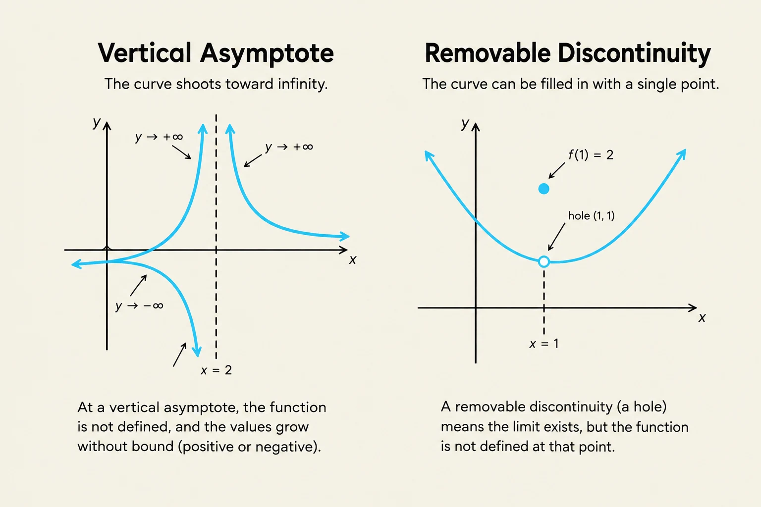
Vertical Asymptotes: These occur at values of x where the denominator is zero and the factor does not cancel out with the numerator. At these points, the function's value approaches ±∞.
Removable Singularities (Holes): If a value of x makes both the numerator and the denominator zero (meaning they share a common factor), that point creates a "hole" in the graph rather than an asymptote.
Beyond vertical behavior, you must identify horizontal asymptotes, which describe the "end behavior" of the function—essentially, what happens to y as x becomes extremely large or extremely small (x→±∞).
This image illustrates two concepts in calculus: vertical asymptotes and removable discontinuities. A vertical asymptote occurs when a function's value approaches infinity as the input approaches a certain value. A removable discontinuity, or a hole, is a point where the function is undefined, but the limit exists.
Exam Tip: Always factor both the numerator and the denominator completely before identifying asymptotes or holes. If a factor cancels, it is a hole; if it remains in the denominator, it is a vertical asymptote.
Solving Polynomial and Rational Inequalities
Inequalities ask you to find the set of x-values that make a statement true (e.g., f(x)>0). Unlike equations, which often have specific point solutions, inequalities usually result in entire intervals of numbers.
To solve these, follow these steps:
Find Critical Values: For polynomial inequalities, find the roots (where the expression equals zero). For rational inequalities, find both the roots of the numerator and the zeros of the denominator.
Test Intervals: Use these critical values to divide the number line into intervals. Pick a "test point" from each interval and plug it into the original expression to see if the result is positive or negative.
Interval Notation: Express your final answer using interval notation (e.g., (−∞,2)∪[5,∞)).
A number line illustrating critical values and intervals, showing where a function is positive or negative.
Exponential and Logarithmic Functions
This section covers functions where the variable is in the exponent or inside a logarithm. The most fundamental concept here is the inverse relationship: an exponential equation can be rewritten as a logarithmic equation and vice versa.
Logarithmic Properties and Equations
To manipulate complex expressions, you must master the three primary logarithmic properties:
Product Property: logb(MN)=logb(M)+logb(N)
Quotient Property: logb(NM)=logb(M)−logb(N)
Power Property: logb(Mp)=p⋅logb(M)
These properties allow you to expand a single logarithm into multiple terms or condense multiple terms into a single logarithm. These skills are essential for solving both exponential equations (by taking the log of both sides) and logarithmic equations (by converting them to exponential form).
Modeling Real-World Scenarios
Exponential and logarithmic functions are powerful tools for modeling natural phenomena:
Growth and Decay: Used to model populations or radioactive decay where the rate of change is proportional to the current amount.
Compound Interest: A specific application of exponential growth used in finance.
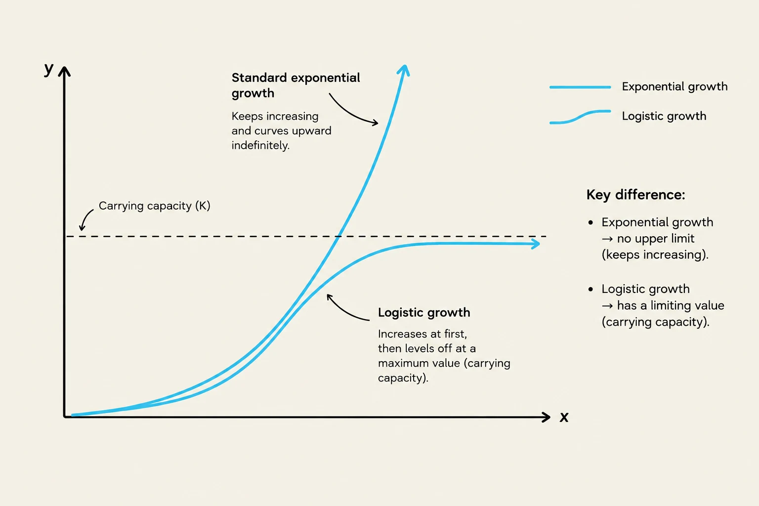
Logistic Growth Model: Unlike simple exponential growth, which goes to infinity, the logistic model accounts for a "carrying capacity"—a limit to how large a population can grow due to environmental constraints.
This graph illustrates the difference between standard exponential growth and logistic growth, highlighting that exponential growth continues indefinitely while logistic growth is limited by a carrying capacity.
Study Strategy: When solving equations, always check for "extraneous solutions." This is especially important with logarithmic equations, as the argument of a logarithm must always be greater than zero.
Keep reading for free.
Create an account to finish this reading and make it part of your study routine.