Understanding Randomness, Probability, and Simulation
Explore the fundamental concepts of randomness, probability, and simulation. Learn how the Law of Large Numbers governs long-term outcomes and how simulations can model real-world random processes, helping to overcome common misconceptions about chance.
Chance is an inescapable part of life. It determines everything from the outcome of a football coin toss to the genetic traits we inherit from our parents. While individual random events can feel chaotic and unpredictable, mathematics allows us to find order within that chaos. By studying the relationship between randomness, probability, and simulation, we can move from guessing about the future to making informed, data-driven inferences.
The Nature of Randomness and Probability
At the heart of this study is the random process. A random process is any mechanism that generates outcomes determined purely by chance. Whether you are rolling a die, tossing a coin, or selecting a person for a survey, the specific result of a single event is unpredictable.
To study these processes, we look at a trial, which is a single repetition of the random process. For example, if you toss a coin ten times, you have conducted ten trials. The result of any single trial is called an outcome.
While we cannot predict a single outcome, we can describe the behavior of the process over time using probability. Probability is a numerical value between 0 and 1 that describes the proportion of times a specific outcome occurs in a very long series of trials.
An outcome with a probability of 0 never occurs.
An outcome with a probability of 1 always occurs.
An outcome with a probability of 0.5 occurs half the time in the long run.
The Law of Large Numbers
A common question in statistics is: "If I know the probability, what should I expect to see in my data?" The answer lies in the distinction between the short run and the long run. In the short run, random processes are erratic. However, they exhibit a regular and predictable pattern over time.
This regularity is guaranteed by the Law of Large Numbers. This principle states that as we observe more and more trials of a random process, the proportion of times a specific outcome occurs (the empirical probability) will approach its theoretical probability.
These graphs illustrate the proportion of heads in coin tosses over increasing numbers of tosses. Graph (a) shows the proportion over 10 tosses, while graph (b) shows it over 500 tosses, demonstrating convergence towards 0.5.
Figure 5.1 shows how the proportion of heads in a coin toss fluctuates wildly during the first few tosses but eventually stabilizes near 0.5 as the number of trials increases.
Human Intuition vs. Reality
Human intuition often fails when dealing with randomness. We tend to expect random sequences to look "even" or "balanced" even in small samples, which leads to two major misconceptions.
The Gambler's Fallacy
Often called the "Law of Averages," this is the misguided belief that future outcomes must "compensate" for past imbalances. For instance, if a coin lands on tails six times in a row, a person might believe a head is "due" to even things out. In reality, random objects like coins have no memory; the probability of the next toss remains exactly the same regardless of what happened before.
Misunderstanding "Runs"
Humans often perceive sequences with long runs—consecutive identical outcomes—as non-random. If you see a sequence like H-H-H-H-H, your intuition might scream that it isn't random. However, in true random processes, runs are surprisingly common and are just as likely to occur as alternating sequences. This is often seen in sports; for example, a basketball player's "hot hand" (a streak of successful shots) is often just a natural run that occurs by chance rather than a change in skill.
Modeling with Simulation
When we want to estimate probabilities or test if a claim is believable, we use simulation. A simulation is a method that imitates a random process so that the simulated outcomes are consistent with real-world outcomes. Simulations are particularly useful when the real-world process is difficult, expensive, or time-consuming to repeat.
The Simulation Process
To conduct a valid simulation, you should follow these three steps:
Describe the process: Define how to perform one trial and what to record at the end of that trial.
Perform many trials: Repeat the process numerous times to gather enough data.
Analyze the results: Use the collected data to answer your question of interest.
Worked Example: The NASCAR Promotion
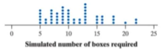
A cereal company claims that five different NASCAR driver cards are equally likely to appear in their boxes. A fan buys 23 boxes and finds she still hasn't collected all five. Is the company lying?
To test this, we can simulate the process:
Trial: Assign a number 1–5 to each driver. Use a random number generator to pick a number. Repeat this until all five numbers have appeared. Record how many numbers it took to get the full set.
Results: After 50 trials, a dotplot might show that it is extremely rare to take 23 or more boxes to complete a set.
A dot plot showing the simulated number of boxes required.
If the simulation shows a $0%$ chance of needing 23 boxes, we have convincing evidence that the cards are not actually equally likely.
AP® EXAM TIP
If you are asked to describe a simulation using a table of random digits, ensure your description is clear enough for someone else to replicate. Every label must be the same length. For example, if labeling students 01 to 95, use two digits for every student. If sampling without replacement, explicitly state that repeated numbers should be ignored.
By combining the theoretical framework of probability with the practical tool of simulation, we can navigate the uncertainty of the world with mathematical confidence.
Keep reading for free.
Create an account to finish this reading and make it part of your study routine.