Understanding Probability: Joint Tables, Conditional Probability, and Independence
Learn to organize data with joint probability tables, calculate conditional probabilities, and determine event independence. Essential for data-driven decision-making.
Probability theory is the backbone of data-driven decision-making. Whether you are analyzing the success of a website redesign or predicting the number of fish a boat will catch, understanding how different events interact is crucial. This article explores how to organize data using joint probability tables, how to calculate conditional probabilities, and how to mathematically prove whether two events are truly independent.
Understanding the Joint Probability Table
When we deal with two different variables simultaneously—such as the type of product defect and the assembly line it came from—we use a joint probability table. This table allows us to see the intersection of two events, showing how often they occur together.
To build a joint probability table from raw counts, you first sum the totals for each row and column. Once you have the totals, you divide each individual cell by the grand total of all observations to convert counts into probabilities.
For example, consider an electronics manufacturer tracking defects across two lines (A and B) and two defect types (Cosmetic and Functional):
Cosmetic defect
Functional Defect
Total
Line A
40
20
60
Line B
30
10
40
Total
70
30
100
By converting these to probabilities (dividing by 100), we find that the probability of a cosmetic defect is P(Cosm)=0.7 and a functional defect is P(Funct)=0.3.
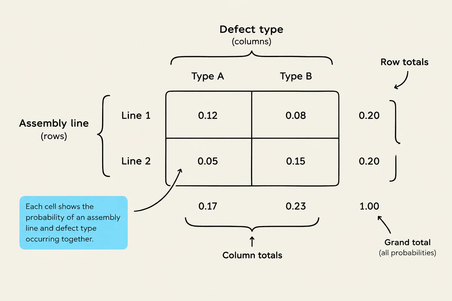
This diagram illustrates the joint probabilities of different defect types occurring on two assembly lines. Each cell represents the probability of a specific assembly line and defect type occurring together, with row and column totals indicating marginal probabilities and a grand total of 1.00 for all probabilities.
Exam Tip: Always check your "Total" row and "Total" column. The sum of all individual joint probabilities in the table must equal 1.0.
Calculating Probabilities of Single and Combined Events
Once your table is constructed, you can answer complex questions about specific groups or combined occurrences.
Probability of a Single Event
To find the probability of a single event (the "marginal probability"), you simply look at the total for that category. For instance, in the e-commerce example where 600 visitors were tracked, we can determine the probability of a visitor viewing a redesign (R) or completing a purchase (P).
The "Or" Rule: Probability of Redesign or Purchase
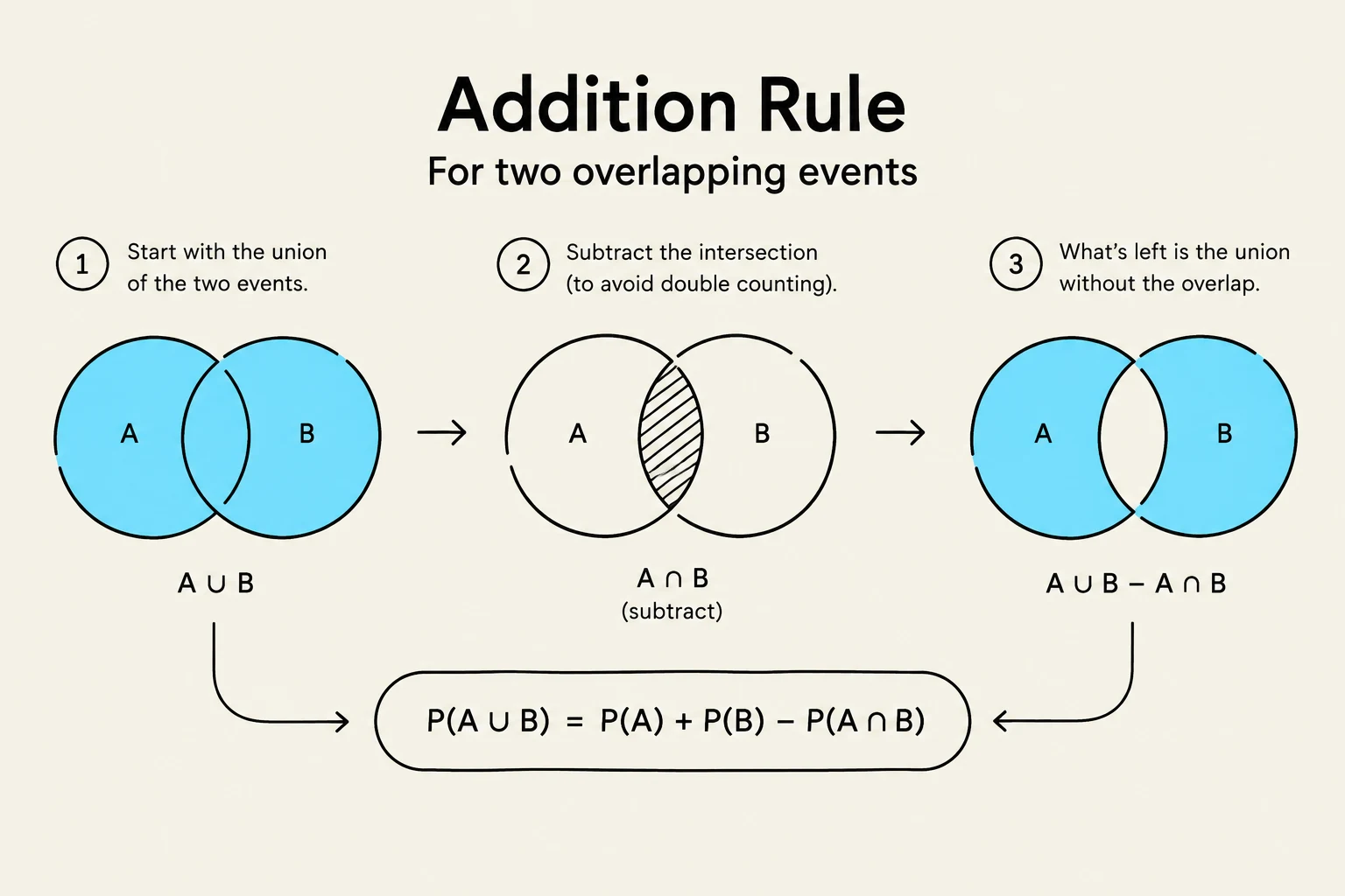
When asked for the probability that a visitor saw the redesign or made a purchase, we use the Addition Rule. We cannot simply add the two individual probabilities because that would count the people who did both twice.
The formula is:
P(A∪B)=P(A)+P(B)−P(A∩B)
Using the e-commerce data:
P(Redesign)=0.5
P(Purchase)=0.25
P(Redesign and Purchase)=0.15
The calculation follows:
P(Redesign or Purchase)=0.5+0.25−0.15=0.6
The Addition Rule for two overlapping events illustrates how to calculate the probability of the union of two events by summing their individual probabilities and subtracting the probability of their intersection to avoid double counting.
Mastering Conditional Probability
Conditional probability is the likelihood of an event occurring given that another event has already happened. This effectively "shrinks" your universe of interest from the entire dataset to a specific row or column.
The notation P(A∣B) is read as "the probability of A given B." The formula is:
P(A∣B)=P(B)P(A∩B)
Worked Examples
Marketing Survey: If a consumer ranked a product as "fair," what is the probability they had "high awareness"? We look only at the "Fair" row in the survey table and divide the "Fair + High Awareness" cell by the total "Fair" row.
E-commerce: What is the probability that a visitor who saw the redesign completed a purchase?
P(Purch∣Red)=0.50.15=0.3
Conversely, for those who saw the old design:
P(Purch∣∼Red)=0.50.1=0.2
Determining if Events are Independent
The most critical question in data analysis is often: "Does one event affect the other?" In probability, two events are independent if the occurrence of one does not change the probability of the other.
The Test for Independence
To mathematically prove independence, you check if the probability of both events happening together is equal to the product of their individual probabilities:
P(A∩B)=P(A)⋅P(B)
If this equation holds true, the events are independent. If not, they are dependent (or "associated").
Applying the Test
Let's return to the e-commerce redesign study:
P(Purchase)=0.25
P(Redesign)=0.5
P(Purchase and Redesign)=0.15
First, calculate the product of the individual probabilities:
P(Purch)⋅P(Red)=0.25⋅0.5=0.125
Now, compare this to the actual joint probability:
0.15=0.125
Because P(A∩B)=P(A)⋅P(B), the events are not independent. In a business context, this suggests that seeing the redesign actually influenced the likelihood of a purchase.
This illustration explains the concept of independent and not independent events using Venn diagrams and probability formulas.
Summary Checklist:
Mutually Exclusive: Events cannot happen at the same time (P(A∩B)=0).
Collectively Exhaustive: The events cover all possible outcomes (P(A∪B)=1).
Independent: One event doesn't change the odds of the other (P(A∩B)=P(A)⋅P(B)).
Keep reading for free.
Create an account to finish this reading and make it part of your study routine.