Understanding Price Elasticity of Demand Using the Midpoint Formula
This content explains the concept of price elasticity of demand, its calculation using the midpoint formula to ensure consistency, and its relationship with total revenue. It covers elastic, inelastic, and unit elastic demand, providing a worked example and a summary table for business strategy.
In economics, understanding how consumers react to price changes is vital for predicting market outcomes. While we know that the Law of Demand dictates an inverse relationship between price and quantity demanded, the real question for businesses and policymakers is: how much does that quantity change? This measurement of responsiveness is known as price elasticity of demand.
Understanding Price Elasticity of Demand
Price elasticity of demand measures the sensitivity of the quantity demanded to a change in price. It is calculated as the percentage change in quantity demanded divided by the percentage change in price:
Price Elasticity of Demand=% change in price% change in quantity demanded
Economists categorize demand into three primary types based on the absolute value of the elasticity coefficient (∣Ed∣):
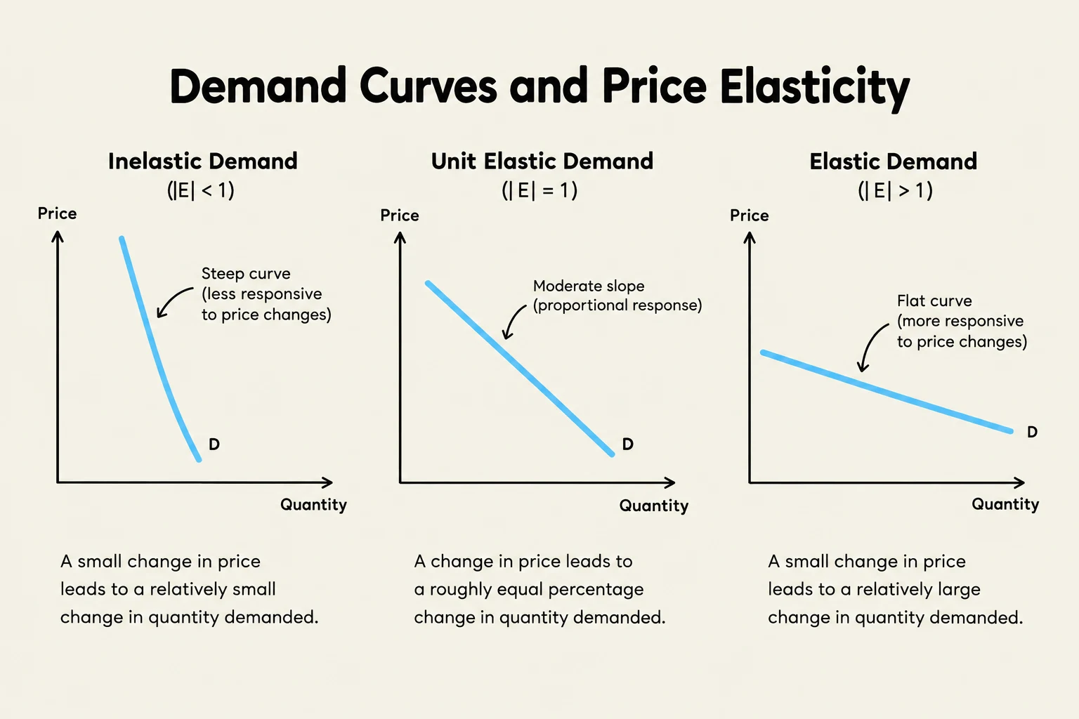
Elastic Demand (∣Ed∣>1): A change in price leads to a relatively large change in quantity demanded.
Inelastic Demand (∣Ed∣<1): A change in price leads to a relatively small change in quantity demanded.
Unit Elastic Demand (∣Ed∣=1): The percentage change in quantity is exactly equal to the percentage change in price.
Exam Tip: Because price and quantity move in opposite directions, the elasticity coefficient is technically negative. However, economists usually drop the minus sign and work with the absolute value.
This illustration shows three types of demand curves: inelastic, unit elastic, and elastic, each with a corresponding explanation of how price changes affect quantity demanded.
The Problem with Standard Percentage Changes
If you use the standard "percentage change" formula—which calculates the change relative to the starting value—you encounter a frustrating mathematical inconsistency.
For example, if a price rises from $$10$to$$20$, the percentage increase is $100%$. However, if the price falls from $20 back to $10, the percentage decrease is only $50%$. This means that calculating elasticity from point A to point B would yield a different result than calculating it from point B to point A. To ensure that the elasticity remains the same regardless of the direction of the price change, economists use the Midpoint Formula.
The Midpoint Formula Explained
The advantage of the midpoint method is that it uses the same base for both increases and decreases, providing a consistent value between any two points. Instead of dividing by the initial value, we divide by the average value of the price and the quantity.
To calculate the percentage change for either price (P) or quantity (Q), use the following mathematics:
% change in X=(2Final Value+Starting Value)Final Value−Starting Value×100
When applying this to the full elasticity formula, we use the average price and the average quantity as our denominators:
Price Elasticity of Demand=(P2+P1)/2P2−P1(Q2+Q1)/2Q2−Q1
Worked Example: Mathematics of Demand Elasticity
Let's apply this to a real-world scenario. Suppose at an initial price of $10, the quantity demanded is 100 units. When the price rises to $20, the quantity demanded falls to 90 units.
Step 1: Calculate the percentage change in quantity demandedChange in Q=90−100=−10Average Q=290+100=95%ΔQ=95−10×100≈−10.5%
Step 2: Calculate the percentage change in priceChange in P=20−10=10Average P=220+10=15%ΔP=1510×100≈66.6%
This illustration demonstrates the calculation of price elasticity of demand using the midpoint formula. It shows a demand curve with two points, (Q1, P1) and (Q2, P2), and details the steps to calculate the percentage change in price and quantity, ultimately determining the elasticity coefficient.
Elasticity and Total Revenue
Understanding elasticity is not just a mathematical exercise; it is a crucial tool for business strategy. Total Revenue (TR) is calculated as Price multiplied by Quantity (P×Q). The relationship between price changes and total revenue depends entirely on the elasticity of the good:
Inelastic Demand: The "price effect" dominates the "quantity effect." If you raise the price, the drop in quantity is so small that total revenue actually increases. (Example: Salt)
Elastic Demand: The "quantity effect" dominates. If you raise the price, the drop in quantity is so significant that total revenue falls. (Example: Airfare)
Unit Elastic Demand: The price and quantity effects perfectly balance each other out, leaving total revenue unchanged.
Summary Table for Decision Making
If Demand is...
A Price Increase will...
A Price Decrease will...
Elastic
Decrease Total Revenue
Increase Total Revenue
Inelastic
Increase Total Revenue
Decrease Total Revenue
Unit Elastic
Leave Total Revenue unchanged
Leave Total Revenue unchanged
By mastering the midpoint formula, you can accurately determine whether a price change will help or hurt a company's bottom line.
Keep reading for free.
Create an account to finish this reading and make it part of your study routine.