Understanding One-Way ANOVA: Logic, Assumptions, and Application
This content explains the fundamental principles of One-Way Analysis of Variance (ANOVA), a statistical method used to compare means across three or more independent groups. It details the decomposition of total variance into between-groups and within-groups components, the calculation and interpretation of the F-ratio
When researchers want to compare the means of several different groups, they often face a dilemma: how can we tell if the differences we see between group averages are "real" (caused by a treatment or factor) or simply the result of random chance? While a t-test can compare two groups, the One-Way Analysis of Variance (ANOVA) is the standard tool for testing three or more independent groups simultaneously.
Despite its name, ANOVA is not actually comparing means directly; instead, it is an Analysis of Variance. It works by breaking down the total variation in a dataset into different sources to see if the variation between groups is significantly larger than the variation within the groups.
Understanding Variance and Error
To understand ANOVA, we must first understand what "variance" represents in a sample. When we take a sample from a population through probability sampling, we rarely get a perfect representation of the population. Even if we draw from a single jar of balls where every ball is labeled "5," a sample might vary if the process isn't perfectly controlled. In real-world research, scores within a single sample vary due to random error.
This error variance stems from several factors:
Measurement error: Inaccuracies in how data is collected.
Individual differences: Natural variations between human subjects (e.g., personality, biology).
We quantify this variation using the Sum of Squares (SS), which measures the total squared deviation of scores from their mean:
SS=∑(X−M)2
Decomposing the Total Sum of Squares
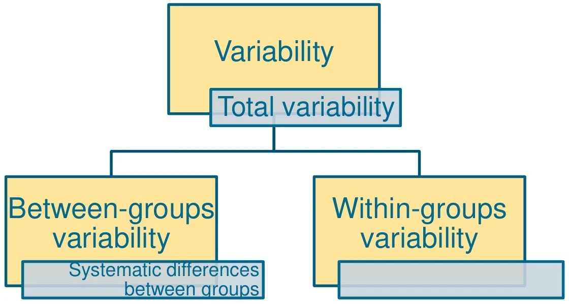
In a One-Way ANOVA, we assume that the total variability in our data ($SS_T$) comes from two distinct sources:
1. Between-Groups Variability (SSBG)
This represents the systematic difference between the group means. If we are testing a new drug, the SSBG captures the effect of that drug. It tells us how much the group means deviate from the overall grand mean.
2. Within-Groups Variability (SSWG or $SS_E$)
Also known as error variance, this represents the random, unsystematic variation among individuals within each specific group. It is the "noise" in our data that exists regardless of whether our treatment works or not.
The relationship is expressed mathematically as:
SST=SSBG+SSWG
A diagram illustrating the components of total variability, distinguishing between between-groups variability and within-groups variability.
The F-Ratio: The Core Logic of ANOVA
The goal of the ANOVA is to determine if the systematic difference (SSBG) is large enough to be distinguished from the random noise (SSWG). We do this by calculating the F-ratio:
F=Variance Within GroupsVariance Between Groups
The logic follows two possible scenarios regarding our hypotheses:
The Null Hypothesis (H0): All population means are equal (μ1=μ2=μ3...). In this case, the only reason the group means would differ is due to random chance. Therefore, the between-groups estimate and the within-groups estimate should be roughly equal, resulting in an F-ratio of approximately 1.
The Research/Alternative Hypothesis (H1): At least one population mean is different. Here, the between-groups estimate includes both random chance and the treatment effect. This makes the numerator larger than the denominator, resulting in an F-ratio greater than 1.
Exam Tip: If you calculate an F-value and it is less than 1, you have likely made a calculation error, as the F-distribution only contains positive values.
Key Assumptions for Validity
For the F-ratio to provide a valid test, four assumptions must be met:
Scale of Measurement: The dependent variable must be interval or ratio scale.
Normality: The populations from which samples are drawn should be normally distributed.
Homogeneity of Variance (Homoscedasticity): All populations should have approximately the same variance.
Independence: All observations must be independent (no paired or matched samples).
Worked Example: The Jury Perception Study
To see this in practice, consider a study investigating how knowledge of a defendant's criminal record affects jury perception.
The Setup:
Researchers assigned 15 volunteers to three groups:
Criminal Record Group: Told the defendant has a history of crime.
Clean Record Group: Told the defendant has a clean record.
No Information Group: Given no info on the record.
The dependent variable was a guilt rating from 1 to 10.
Hypotheses:
H0:μ1=μ2=μ3 (Criminal record knowledge has no effect on guilt ratings).
H1: At least one mean is different.
The Decision Process:
After calculating the Sum of Squares for both between-groups and within-groups, the researcher determines the Degrees of Freedom (df):
dfbetween=number of groups−1=3−1=2
dfwithin=total participants−number of groups=15−3=12
Using an F-table at the α=.05 significance level, the researcher finds the critical value for F(2,12) is 3.89.
Conclusion:
If the calculated Fstat>3.89, we reject the null hypothesis and conclude that the criminal record information significantly changed jury perceptions.
If Fstat≤3.89, we fail to reject the null hypothesis, concluding there is no evidence that the record information affected the ratings.
Keep reading for free.
Create an account to finish this reading and make it part of your study routine.