Understanding OLS Estimator Variance and Homoskedasticity
This content explains the variance of Ordinary Least Squares (OLS) estimators, the crucial assumption of homoskedasticity, and its implications for statistical inference. It details how error variance, variation in regressors, and sample size affect estimator precision, and discusses the estimation of error variance an
In econometrics, estimating the relationship between variables is only half the battle. Once we have calculated our Ordinary Least Squares (OLS) coefficients, we must ask: how much can we trust them? The precision of our estimates is determined by their variance. Understanding the factors that influence this variance—and the assumptions required for our statistical tests to be valid—is essential for any meaningful empirical analysis.
The Variance of the OLS Estimator
The variance of an OLS estimator measures the spread or uncertainty of the coefficient estimates. If we were to take many different samples from the same population, the variance tells us how much our estimated β^ values would fluctuate from sample to sample.
Under the classical assumption of homoskedasticity, the conditional variance of the error term is constant across all observations, expressed as:
Var(ui∣xi)=σ2
When this assumption holds, the variances for the intercept (β^1) and the slope (β^2) are defined by specific formulas:
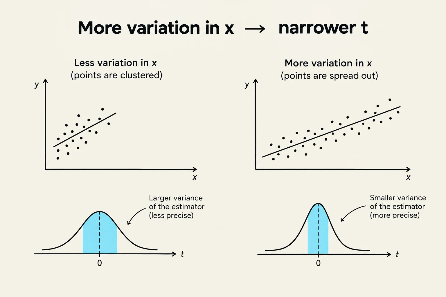
This illustration demonstrates how increased variation in the independent variable (x) leads to a narrower distribution of the estimator (t), indicating greater precision. The left side shows less variation in x with clustered points, resulting in a larger variance of the estimator (less precise). The right side shows more variation in x with spread-out points, leading to a smaller variance of the estimator (more precise).
From these formulas, we can derive three critical insights regarding the precision of our slope estimate (β^2):
Error Variance (σ2): A larger error variance increases the variance of the estimator. This reflects greater "noise" or uncertainty in the relationship between y and x.
Variation in x: An increase in the total variation of the regressor x (the denominator) decreases the variance of β^2. Essentially, more variation in x provides more information about the underlying relationship.
Sample Size (n): As the sample size increases, the total variation in x typically increases, which subsequently reduces the variance of the estimator.
Estimating σ2 and Standard Errors
In real-world research, the true population error variance σ2 is unknown. We must instead use an unbiased estimator, denoted as s2:
s2=n−k1∑i=1nu^i2
Here, k represents the number of β parameters in the model, and n−k represents the degrees of freedom. Once we have estimated s2, we can calculate the standard error of our coefficients by taking the square root of the estimated variance. These standard errors are the foundation for calculating t-statistics and determining p-values to test for statistical significance.
Exam Tip: Remember that the degrees of freedom (n−k) decreases as you add more independent variables to your model. This is the "penalty" you pay for increasing model complexity.
Homoskedasticity vs. Heteroskedasticity
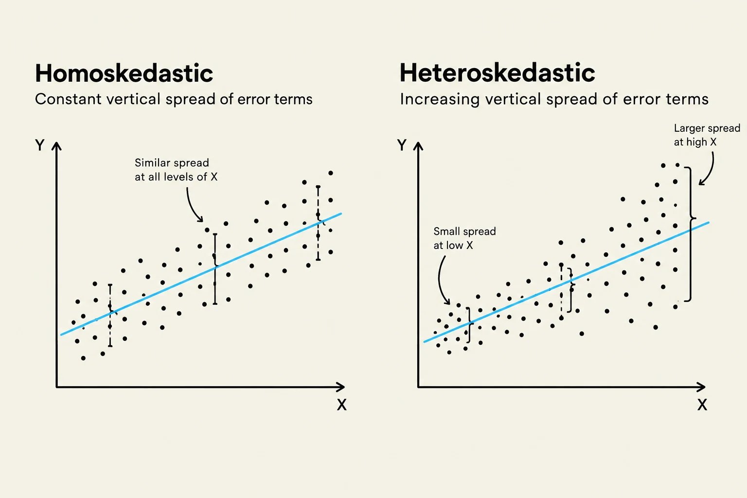
The validity of the standard OLS variance formulas depends entirely on the assumption of homoskedasticity—the idea that the "spread" of the error term is constant.
When this assumption is violated, we encounter heteroskedasticity. This occurs when the conditional variance of the error term depends on the value of an independent variable.
Comparison of homoskedasticity and heteroskedasticity in statistical models, illustrating constant versus increasing vertical spread of error terms.
A classic example is the relationship between income and savings. Families with very low incomes have little discretion; they must spend most of their income on necessities, leading to low variation in savings. However, high-income families have much more discretion—some may save aggressively while others spend lavishly—leading to much higher variation in savings behavior.
If heteroskedasticity is present, the standard OLS formulas for variance become invalid. While the β^ estimates themselves may remain unbiased, the calculated standard errors will be incorrect, which can lead to misleading t-statistics and incorrect conclusions about whether a variable is statistically significant.
Omitted Variable Bias and Error Term Correlation
A major threat to the reliability of OLS is the violation of the Zero Conditional Mean assumption, which states that $E[u|x] = 0$. This assumption implies that the error term u is not correlated with the regressor x (i.e., $Cov(x, u) = 0$).
If we omit a variable from our model that is both a determinant of y and correlated with x, we encounter omitted variable bias. In this scenario, the effect of the omitted variable is "soaked up" by the error term, creating a correlation between x and u.
Worked Example: Education and Wages
Consider a model: wage=β1+β2educ+e.
If we want to measure the effect of education on wages, we must ensure that the error term e (which contains unobserved factors like "innate ability") is not correlated with education.
However, if individuals with higher innate ability tend to seek more education, then e and educ are correlated. In this case, the OLS estimate β^2 will not just capture the effect of education; it will also capture part of the effect of innate ability, leading to a biased estimate of the true return to schooling.
This diagram illustrates the relationship between ability, education, and an outcome variable 't', highlighting the concept of an omitted variable bias in statistical analysis.
Summary Table: Impact of Assumptions
Assumption
If Violated...
Result
$E[u
x] = 0$
Omitted Variable Bias
\hat{\beta}$ is biased and inconsistent | | Var(u|x) = \sigma^2∣Heteroskedasticity∣\hat{\beta}$ is unbiased, but standard errors are wrong |
Keep reading for free.
Create an account to finish this reading and make it part of your study routine.