This guide explains the fundamental principles of motion under constant acceleration in physics, covering vectors, kinematic equations, and projectile motion. It details how to analyze the horizontal and vertical components of motion, initial conditions, and final velocity, with examples like calculating maximum height
In physics, describing how an object moves through space requires more than just knowing its speed. We must understand how that speed changes over time and how its position evolves. When an object experiences a steady, unchanging rate of change in velocity, we call this constant acceleration. This principle is fundamental to understanding everything from a ball being kicked in a football game to a fish swimming through the ocean.
The Foundation: Vectors and Components
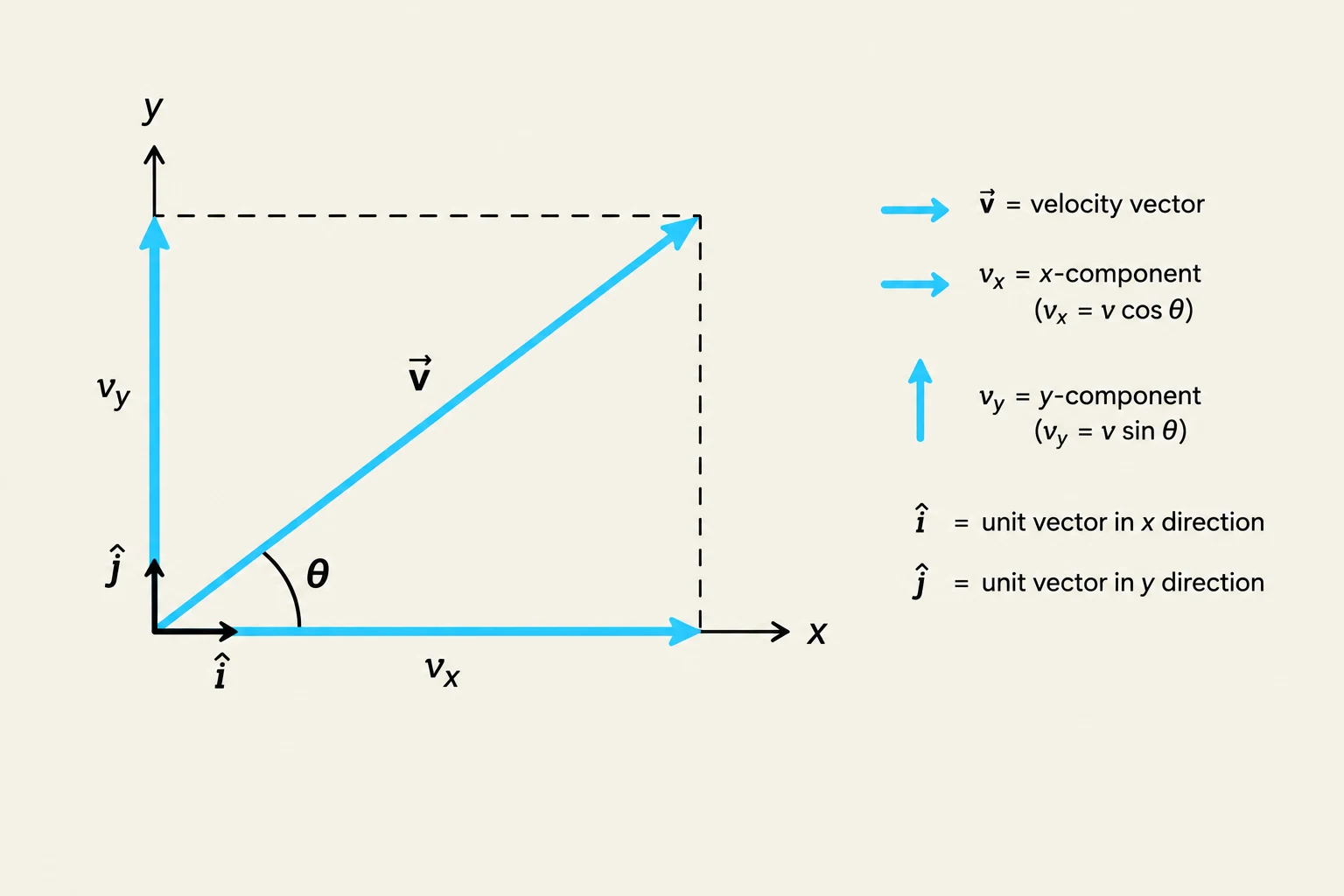
To analyze motion in two or three dimensions, we cannot rely on simple numbers; we must use vectors. A position vectorr describes where an object is located relative to an origin. As the object moves, this vector changes, tracing a path through space. Similarly, the velocity vectorv represents the instantaneous rate of change of position, indicating both how fast the object is moving and in what direction.
In most textbook problems, we break these vectors into acceleration components along the x and y axes. We use unit vectorsi^ and j^ to denote these directions. For example, a velocity can be written as:
v=vxi^+vyj^
A diagram illustrating the decomposition of a velocity vector into its x and y components, along with the definitions of unit vectors in the x and y directions.
When dealing with projectile motion—such as a tennis ball launched at an angle—the initial velocity is often split using trigonometry:
vix=vicosθ
viy=visinθ
Analyzing Constant Acceleration
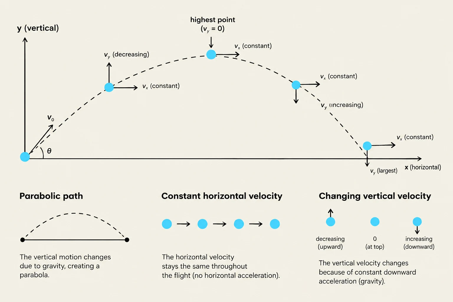
When acceleration is constant, the velocity changes by the same amount every second. The direction of acceleration is crucial. In projectile motion, we often ignore air resistance, meaning the only acceleration is gravity, which acts strictly in the downward direction (the negative y direction). This means the horizontal component of acceleration is zero (ax=0), resulting in a constant horizontal velocity.
To solve these problems, you must identify the initial conditions. These are the values of position and velocity at the exact moment the motion begins (t=0). Without knowing the initial speed (vi), the launch angle (θ), and the starting position ($x_i, y_i$), you cannot predict the future state of the particle.
Exam Tip: Always check if the acceleration is truly constant. If a problem mentions "air resistance," the acceleration is no longer constant because it changes based on the object's speed, and these standard kinematic equations will no longer be accurate.
Kinematic Equations and Final Velocity
By combining the initial conditions with the constant acceleration, we can derive equations to find the final velocity (vf) or the final position at any time t.
For the vertical direction (y), the velocity at any time is:
vy=viy+ayt
Since gravity (g≈9.8 m/s2) acts downward, we substitute ay=−g:
vy=visinθ−gt
The vertical position is given by:
y=yi+(visinθ)t−21gt2
This diagram illustrates projectile motion, showing how horizontal velocity remains constant while vertical velocity changes due to gravity, resulting in a parabolic path.
Worked Example: Maximum Height
Suppose a tennis ball is launched at 30 m/s at an angle θ. To find the maximum height (h), we first find the time it takes to reach the peak. At the peak, the vertical component of velocity is zero (vy=0):
0=visinθ−gt⟹t=gvisinθ
Substituting this time back into the position equation:
h=2g(visinθ)2
Notice that if you double the initial speed (vi), the maximum height does not just double—it quadruples, because the velocity term is squared.
Summary of Motion Characteristics
Motion Aspect
Horizontal Component (x)
Vertical Component (y)
Acceleration
ax=0 (Constant velocity)
ay=−g (Constant acceleration)
Velocity
vx=vix (Stays the same)
vy changes linearly with time
Key Feature
Determines the Range (R)
Determines Max Height (h) and Time of Flight
By mastering these components, you can decompose any complex 2D motion into two simple 1D problems, making even the most difficult projectile trajectories easy to calculate.
Keep reading for free.
Create an account to finish this reading and make it part of your study routine.