Understanding Function Transformations and Algebraic Analysis
Explore function transformations, including vertical scaling, reflections, and translations, and learn how to perform algebraic analysis of graphs, covering domain, range, intercepts, intervals of increase/decrease, extrema, and end behavior.
In mathematics, functions are more than just static equations; they are dynamic relationships that can be shifted, stretched, and manipulated to model real-world phenomena. By understanding how to transform a parent function—the simplest form of a function family—and how to perform a rigorous algebraic analysis of its graph, you can unlock a deeper understanding of how variables interact. This article explores the mechanics of function transformations and the essential tools used to analyze the behavior of functions.
Function Transformations
A transformation is a change made to a parent function f(x) to create a new function g(x). Most transformations can be summarized by the general form:
g(x)=a⋅f(x−h)+k
Each parameter ($a, h, k$) serves a specific purpose in altering the graph's position or shape.
Vertical Scaling and Reflections
The coefficient a controls the vertical aspect of the graph:
Vertical Stretch: If ∣a∣>1, the graph is stretched away from the x-axis.
Vertical Compression: If 0<∣a∣<1, the graph is compressed toward the x-axis.
Reflection along the x-axis: If a is negative, the entire graph is flipped upside down.
Translations (Shifts)
The parameters h and k move the graph without changing its shape:
Horizontal Translation (h): This shifts the graph left or right. Note the sign convention: (x−h) shifts the graph to the right, while (x+h) shifts it to the left.
Vertical Translation (k): This shifts the graph up or down. A positive k moves the graph up, and a negative k moves it down.
Exam Tip: Tracking Points
When a point (x,y) exists on the parent function, you can find its new location on the transformed function by applying the changes to the coordinates. The new x-coordinate becomes x+h (to counteract the subtraction in the formula), and the new y-coordinate becomes a(y)+k.
For example, if we have a parent function f(x)=x and we want to transform it into g(x)=−x−4+2, we identify the following:
a=−1 (reflection along the x-axis)
h=4 (shift right 4 units)
k=2 (shift up 2 units).
Algebraic Analysis of Graphs
Once a function is transformed, we use algebraic analysis to describe its specific properties. This involves looking at intervals, specific points of interest, and the overall "flow" of the graph.
Domain and Range
The domain is the set of all possible input values (x), while the range is the set of all possible output values (y). It is important to note that transformations directly impact these sets. A horizontal shift (h) will change the domain, while vertical scaling (a) and vertical shifts (k) will change the range.
Intercepts
Intercepts are the points where the graph crosses the axes:
x-intercepts: The points where the graph crosses the x-axis, occurring when f(x)=0.
y-intercept: The point where the graph crosses the y-axis, occurring when x=0.
Intervals of Increase, Decrease, and Constant Behavior
We describe the movement of a function using x-intervals:
Increasing Interval: The intervals where the graph slopes upward as you move from left to right.
Decreasing Interval: The intervals where the graph slopes downward.
Constant Interval: The intervals where the graph is a flat, horizontal line.
Extrema: Maximums and Minimums
Extrema are the "peaks" and "valleys" of a function. They are categorized into two types:
Relative (Local) Extrema: A relative maximum is a local peak, and a relative minimum is a local valley.
Absolute (Global) Extrema: The absolute maximum is the highest point on the entire graph, and the absolute minimum is the lowest point.
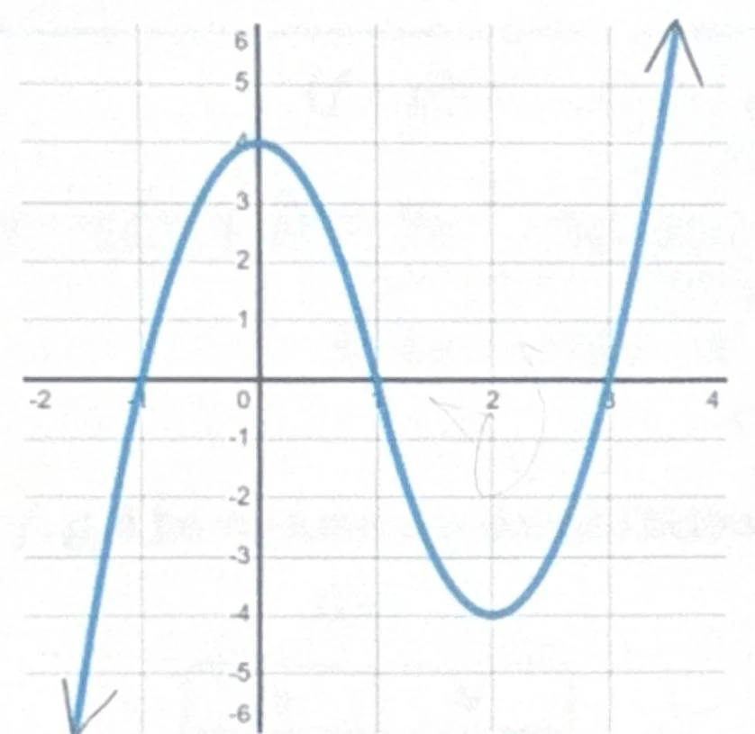
A graph showing a cubic function with x-axis values from -2 to 4 and y-axis values from -6 to 6.Figure 1: An example of a cubic function showing various analytical properties.
End Behavior
End behavior describes what happens to the function as x moves toward positive or negative infinity. This is formally expressed using limits:
limx→∞f(x)andlimx→−∞f(x)
For example, a function might approach infinity (∞) or negative infinity (−∞) as x grows larger or smaller.
Function Operations and Composition
Beyond analyzing single functions, we can combine them through operations or composition.
Basic Operations
Given two functions f(x) and g(x), we can perform addition, subtraction, multiplication, and division:
Addition: (f+g)(x)=f(x)+g(x)
Subtraction: (f−g)(x)=f(x)−g(x)
Multiplication: (f⋅g)(x)=f(x)⋅g(x)
Division: (gf)(x)=g(x)f(x).
Function Composition
Composition involves nesting one function inside another, denoted as (f∘g)(x), which means $f(g(x))$. In this process, the output of the inner function g(x) becomes the input for the outer function f(x).
Contextual Application
Composition is often used to link multiple variables. For instance, if V(t) represents the number of visitors based on temperature, and F(x) represents the amount of food needed based on the number of visitors, then the composition (F∘V)(t) represents the amount of food needed in terms of the daily temperature.
Keep reading for free.
Create an account to finish this reading and make it part of your study routine.