Understanding Curvilinear Motion: Normal and Tangential Acceleration
Explore the principles of curvilinear motion, focusing on how to analyze acceleration using tangential and normal components. Learn about velocity, the hodograph, and the n-t coordinate system with practical examples.
When a particle moves along a straight line, we describe its motion using simple linear coordinates. However, in the real world, objects rarely move in perfectly straight lines. They follow curves—from a car navigating a highway interchange to a satellite orbiting the Earth. This type of movement is known as curvilinear motion.
To analyze these complex paths, engineers often move away from standard $x, y, z$ rectangular coordinates and instead use a coordinate system that "follows" the particle along its path. This system uses unit vectors that are always tangent and normal to the curve, allowing us to separate the acceleration into components that describe how the speed changes and how the direction changes.
Understanding Curvilinear Motion
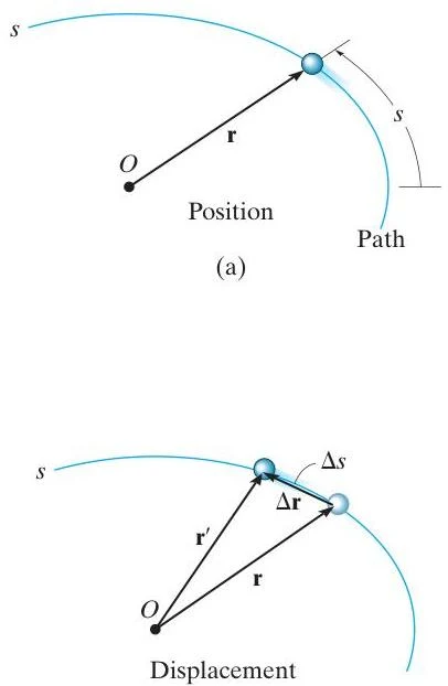
Curvilinear motion occurs when a particle moves along a space curve defined by a path function s(t). The position of the particle is represented by a position vector r, which changes in both magnitude and direction as the particle progresses.
This diagram illustrates position and displacement vectors for an object moving along a curved path. Part (a) shows the position vector 'r' from the origin 'O' to the object, and the path length 's'. Part (b) depicts the change in position, or displacement vector 'Δr', between two points on the path, with corresponding path length change 'Δs'.
Velocity and the Tangent
The instantaneous velocity v is the time derivative of the position vector v=dtdr. A fundamental property of velocity in curvilinear motion is that the velocity vector is always tangent to the path. The magnitude of this velocity vector, v, is the speed, which can be calculated by differentiating the arc length s with respect to time:
v=dtds
Acceleration and the Hodograph
Acceleration a is the time derivative of velocity a=dtdv. Unlike velocity, the acceleration vector is not necessarily tangent to the path. Because a curved path requires a change in the direction of the velocity vector, the acceleration must "swing" toward the inside or the concave side of the curve.
If we plot the velocity vectors with their tails at a fixed point, the resulting curve is called a hodograph. The acceleration vector is always tangent to this hodograph, even if it is not tangent to the actual path of motion.
The n−t Coordinate System
To simplify the analysis of acceleration, we define a local coordinate system at any point along the path. This system consists of two perpendicular unit vectors:
Tangential Unit Vector (ut): This vector is always tangent to the path at the particle's current position.
Normal Unit Vector (un): This vector is perpendicular to the tangential vector and points toward the center of curvature (the "inside" of the curve).
In three-dimensional spatial motion, a third axis called the binormal axis (ub) is used to complete the coordinate system. The plane formed by the tangential and normal vectors is known as the osculating plane.
Radius of Curvature
The "tightness" of a curve at any given point is described by the radius of curvature, denoted as ρ. A smaller ρ indicates a sharper turn, while a larger ρ indicates a flatter, more gradual curve.
Components of Acceleration
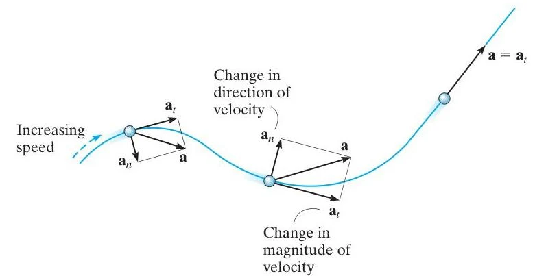
By using the n−t axes, we can decompose the total acceleration vector a into two distinct physical components:
1. Tangential Acceleration (at)
The tangential component represents the rate of change of the speed (the magnitude of velocity). It tells us how much the particle is speeding up or slowing down along its path.
at=v˙=dtdv
2. Normal Acceleration (an)
The normal component represents the rate of change in the direction of the velocity. This is also frequently called centripetal acceleration. Even if a particle moves at a constant speed, it will still have a normal acceleration as long as it is turning. It is calculated using the speed and the radius of curvature:
an=ρv2
Exam Tip: If a problem states a particle is moving at a constant speed, you can immediately set the tangential acceleration at=0. However, do not assume the total acceleration is zero; the normal acceleration an will still exist if the path is curved.
The total magnitude of the acceleration is found using the Pythagorean theorem:
a=at2+an2
This diagram illustrates the tangential and normal components of acceleration for an object moving along a curved path. The tangential acceleration (at) is responsible for changes in speed, while the normal acceleration (an) is responsible for changes in the direction of velocity.
Worked Example: Analyzing a Curved Path
Problem: A car is traveling along a circular track with a radius of ρ=40 m. At a certain instant, the car's speed is v=20 m/s and its speed is increasing at a rate of at=2 m/s2. Determine the magnitude of the car's total acceleration.
Solution:
Identify the components:
The tangential acceleration is given: at=2 m/s2.
The speed is v=20 m/s.
The radius of curvature for a circular path is the radius itself: ρ=40 m.