This content explains statistical power, its relationship to Type I and Type II errors, and the four key variables that influence it: alpha, effect size, variance, and sample size. It details a priori sample size estimation for planning studies and post-hoc power analysis for interpreting results, emphasizing the impor
In the world of research, we are essentially trying to estimate the truth. Because we cannot study every single person in a population, we use samples and statistical tests to make inferences. However, even with perfect math, there is always a risk of being wrong. One of the most critical concepts in ensuring our research is meaningful is statistical power: the probability that a study will correctly detect a true effect or difference when one actually exists.
If a study has low power, it might fail to find a difference that is actually there, leading to a Type II error (failing to reject a false null hypothesis). To avoid this, researchers must understand the mechanics of power before they ever begin collecting data.
The Four Pillars of Power
Statistical power is not a random number; it is mathematically determined by the interplay of four interconnected variables. If you change one of these pillars, the others must shift to maintain the same level of power.
1. Alpha (α)
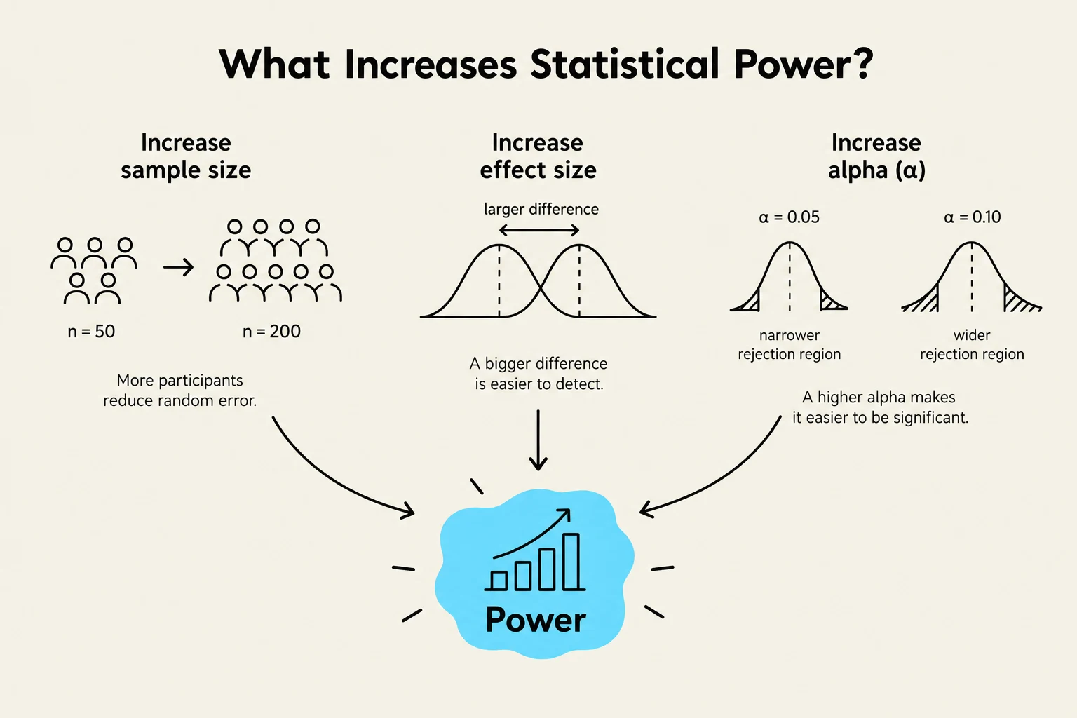
Alpha is the significance level, representing the probability of committing a Type I error—rejecting a null hypothesis that is actually true (a "false positive"). While we often set α at 0.05, it directly influences power. A more stringent (smaller) alpha makes it harder to reject the null hypothesis, which can decrease your power.
2. Effect Size
Effect size refers to the magnitude of the difference or relationship being studied. Imagine trying to detect a difference in height between two groups: it is much easier to detect a 10-inch difference (large effect size) than a 0.1-inch difference (small effect size). Larger effects are easier for statistical tests to "see," thereby increasing power.
3. Variance
Variance represents the "noise" or variability within your data. If you are measuring weight in a group of identical twins, the variance will be low. If you are measuring weight in a random group of adults, the variance will be high. High variance obscures the "signal" of the effect, making it harder to detect and thus reducing power.
4. Sample Size (n)
Sample size is the number of observations or participants in your study. This is the primary lever researchers can control. As the sample size increases, the precision of your estimate improves, and the ability to detect an effect increases.
This diagram illustrates factors that increase statistical power, including increasing sample size, increasing effect size, and increasing alpha (significance level).
A Priori Power Analysis: Planning for Success
The most responsible way to use power is a priori, which means performing the analysis before the study begins. The goal of an a priori analysis is sample size estimation: determining exactly how many participants are needed to ensure the study is robust enough to detect a meaningful difference.
To perform this, researchers typically set a target power—commonly $80%$ (0.80), which is considered the minimal acceptable threshold in most fields. They then input their chosen alpha, their expected effect size, and their anticipated variability into software like G*Power or SPSS to solve for n.
Exam Tip: If a question asks when you should perform sample size estimation, the answer is a priori (before data collection).
Moving Beyond "Lazy" Effect Sizes
A common mistake in a priori planning is using "lazy" methods, such as relying solely on generic standardized effect sizes like Cohen's d (a mean difference divided by the standard deviation). While Cohen's d provides a general sense of magnitude (small, medium, or large), it may not be clinically relevant.
A much more robust approach is to power a study to detect the Minimal Clinically Important Difference (MCID). The MCID is the smallest change in a treatment outcome that a patient would actually perceive as beneficial. By using the MCID and estimating variance from previous literature, researchers ensure their study is designed to find differences that actually matter to patients, not just differences that are mathematically significant.
Post-hoc Power Analysis: Interpreting Results
Post-hoc power analysis occurs after a study is completed. This is primarily used by consumers of research when a study fails to reject the null hypothesis (i.e., the results were not statistically significant).
If a study finds no difference, a post-hoc calculation can help determine if the result was truly due to a lack of effect, or if the study was simply "underpowered"—meaning it didn't have enough participants or precision to see the effect.
Caution: Post-hoc power should be interpreted with care. Some experts argue that observed post-hoc power adds little value; instead, you should focus on effect estimates and confidence intervals.
The Gold Standard: Confidence Intervals (CI)
Rather than relying solely on a p-value or a post-hoc power number, the most effective way to evaluate a "negative" trial (one that found no statistical significance) is through Confidence Intervals (CI).
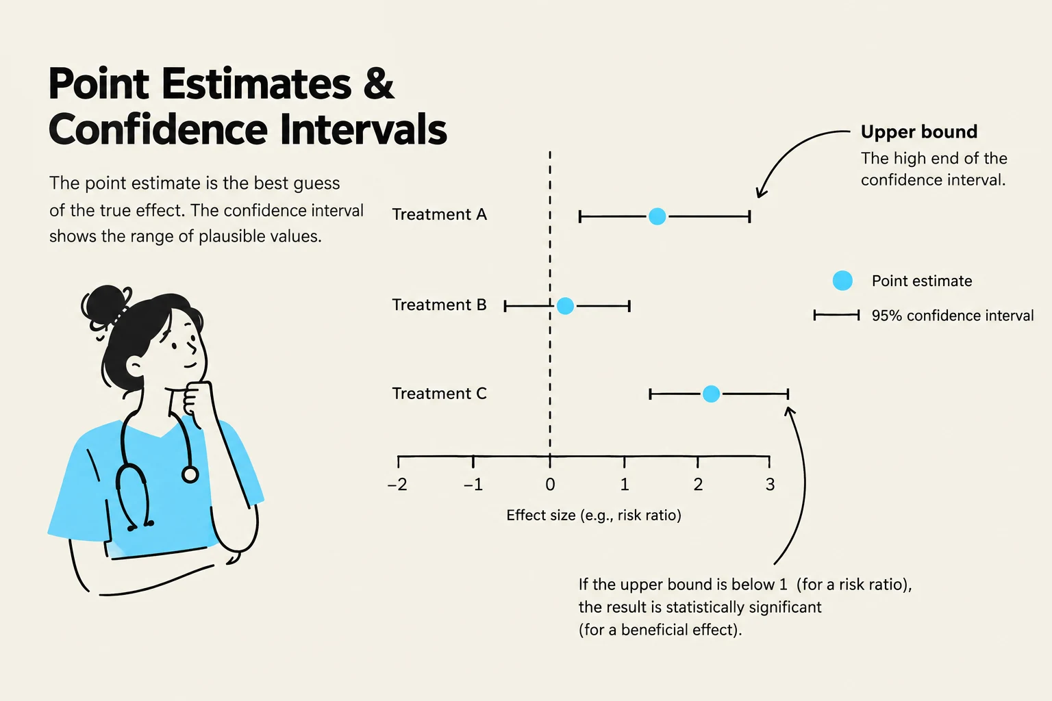
When you look at a 95% CI, you are looking at the range of values within which we are 95% confident the true effect lies. To determine if a study is truly "negative" or just "underpowered," you must compare the upper bound of the CI to the MCID.
Underpowered (Imprecise): If the 95% CI is very wide and includes the MCID, the study is inconclusive. We cannot say there is no effect; we can only say our estimate was too imprecise to rule out a clinically important difference.
Definitively Negative (Precise): If the 95% CI is narrow and even its upper bound is still below the MCID, the study is a "definitively negative trial". This means that even if there is an effect we missed, it is so small that it wouldn't matter to the patient.
Worked Example: The Knee Arthroscopy Study
Consider a landmark study in the New England Journal of Medicine regarding knee arthroscopy for osteoarthritis. The study found no statistically significant difference in pain between real surgery and a placebo (sham) surgery.
Critics might claim the study was underpowered. However, the researchers showed that the 95% confidence intervals for the difference in pain were very small. Even the upper bound of those intervals was much lower than the MCID. Therefore, the researchers could confidently state that the treatment was not only statistically insignificant but also clinically irrelevant.
This illustration explains point estimates and confidence intervals, which are statistical concepts used to estimate the true effect of a treatment or intervention. The graph shows the point estimate (the best guess of the true effect) and the 95% confidence interval (the range of plausible values) for three different treatments (A, B, and C). It also illustrates how to interpret the results for statistical significance based on the upper bound of the confidence interval.
Keep reading for free.
Create an account to finish this reading and make it part of your study routine.