Probability Definitions and Distribution Functions
Explore the fundamental concepts of probability, including its definition, the range of probability values, and the distinction between discrete and continuous random variables. Learn about Probability Mass Functions (PMF) for discrete variables and Probability Density Functions (PDF) for continuous variables, includin
In the study of statistics and data analysis, we often encounter uncertainty. Whether we are measuring the viscosity of oil in a distillation column or predicting the age of trees in a forest, measurements are rarely identical due to random variations. To manage this uncertainty, we use the concept of probability to quantify how likely it is that a specific outcome will occur.
Probability Definition
The probability (P) of an event (X) is a mathematical measure of the likelihood that the event will occur. Probability is strictly constrained within a specific range:
0≤P(X)≤1
If the probability of an event is 0, it is considered impossible. Conversely, if the probability is 1, the event is certain to occur.
Random Variables
A random variable is a variable subject to random variations, meaning it can take on multiple different values, each with an associated probability. Based on the nature of these values, we categorize random variables into two primary types: discrete and continuous.
Discrete Random Variables
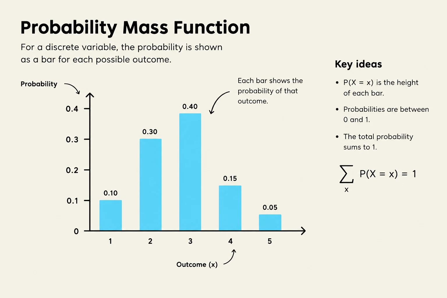
Discrete random variables involve outcomes that are countable or distinct. Examples include the number of scratches on a surface, the number of plant shutdowns, or the result of a coin toss. Because these outcomes are separate points, we use a Probability Mass Function (PMF) to describe them.
A fundamental rule of the PMF is that the sum of all individual probabilities for all possible outcomes must equal exactly 1:
∑all XP(X)=1
A probability mass function graph illustrating the probability of discrete outcomes.
Exam Tip: When working with discrete variables, always ensure that your individual probabilities are non-negative and that their total sum equals 1. If they do not, you have likely missed an outcome or made a calculation error.
Continuous Random Variables
Continuous random variables involve values that can take any value within a given range or interval. Unlike discrete counts, these are often measurements, such as temperature, pressure, the angle of a spinning top, or the age of trees in a forest.
Because there are an infinite number of possible values between any two points, we cannot assign a probability to a single, exact point. Instead, we use a Probability Density Function (PDF), denoted as f(x), to describe the distribution.
The Probability Density Function (PDF)
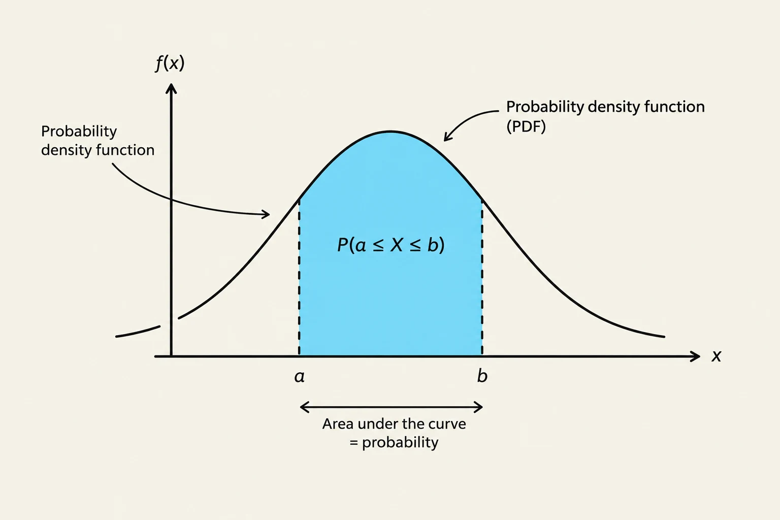
The PDF represents how densely a population is distributed around specific values. While the height of the function f(x) at a certain point indicates the relative likelihood of the variable falling near that value, the function itself does not represent a probability. Instead, probability is found by calculating the area under the curve between two points.
For a function to be a valid PDF, it must satisfy two essential properties:
Non-negativity: The value of the PDF is never negative (f(x)≥0).
Total Area: The total area under the full curve must equal 1:
∫−∞∞f(x)dx=1
A probability density function (PDF) graph illustrating the probability of a random variable X falling between values a and b, represented by the area under the curve.
Calculating Probability in Continuous Distributions
To find the probability that a variable X falls between two values, a and b, we calculate the definite integral of the PDF:
P(a≤X≤b)=∫abf(x)dx
An important consequence of this is that the probability of a continuous variable taking on one specific, exact value is zero:
P(a≤X≤a)=∫aaf(x)dx=0
Worked Example: Exponential Distribution
Consider the diameter of copper wires produced in a plant. The thickness X follows an exponential distribution with the following PDF:
f(x)={20e−20(x−12.5)0x≥12.5x<12.5
Question: What proportion of wires must be discarded if thicknesses greater than 12.6 mm are unacceptable?
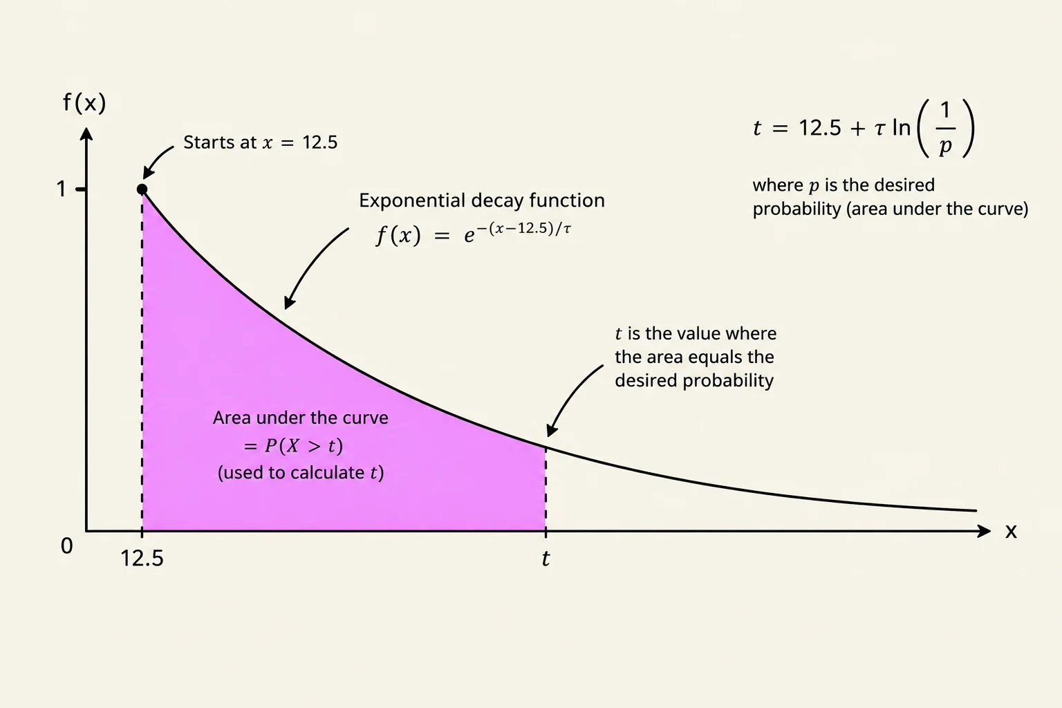
To solve this, we find the area under the curve from 12.6 to infinity:
P(X>12.6)=∫12.6∞20e−20(x−12.5)dx=[−e−20(x−12.5)]12.6∞=0−(−e−20(12.6−12.5))=e−20(0.1)=e−2≈0.135
Thus, approximately $13.5%$ of the wires would be discarded.
This graph illustrates an exponential decay function, showing how the probability decreases over time. It highlights the concept of area under the curve representing probability and provides a formula to calculate a specific time 't' based on a desired probability 'p'.
Keep reading for free.
Create an account to finish this reading and make it part of your study routine.