Normal-Curve Tail Probabilities and the Single-Sample Z Test
Learn about z-scores, normal-curve tail probabilities, and how to conduct a single-sample z test to determine if a sample mean differs significantly from a population mean.
In statistics, we often encounter a fundamental question: is an observed result a product of random chance, or does it represent a genuine departure from what we expected? To answer this, we rely on the properties of the normal distribution to quantify how "unusual" a specific value or sample mean is. By using z-scores and tail probabilities, we can move from simple observations to formal statistical inference through the Single-Sample Z Test.
Understanding the Z-Score
Before we can calculate probabilities, we must understand the z-score. A z-score expresses a value's distance from the mean in units of standard deviation. It allows us to compare different types of data—such as grades, income, or height—on a single, common scale.
The formula for a z-score is:
z=σx−μ
Where x is the observed value, μ is the population mean, and σ is the population standard deviation.
A z=0 means the value is exactly at the mean.
A z=+1 means the value is one standard deviation above the mean.
A z=−1 means the value is one standard deviation below the mean.
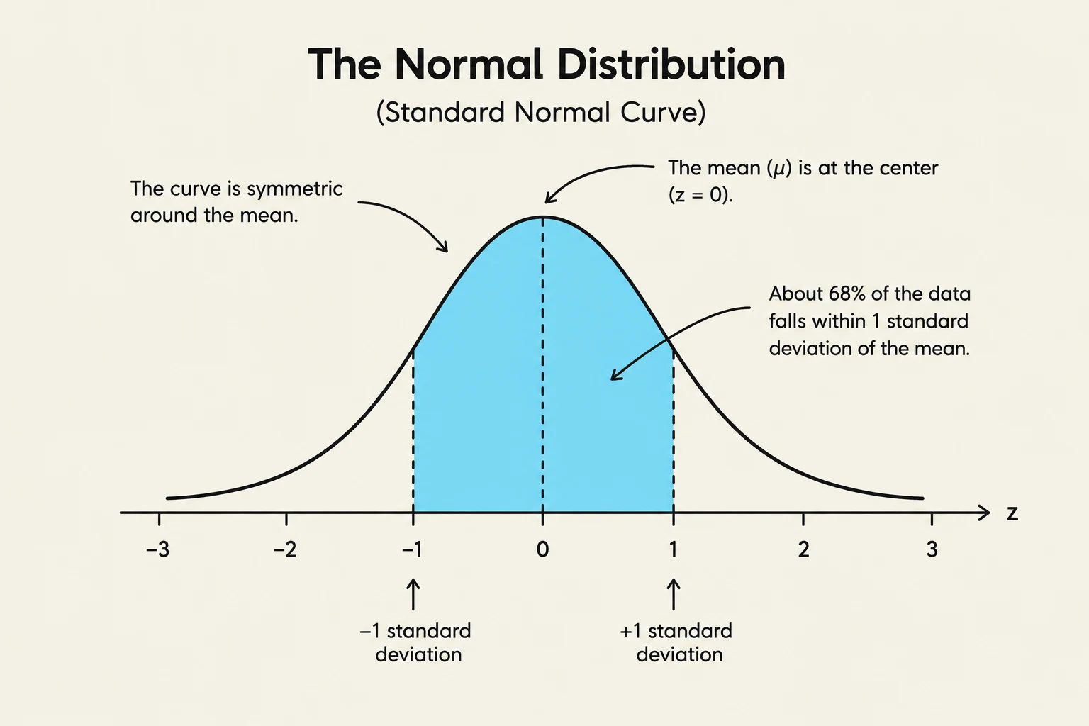
The image illustrates the normal distribution, also known as the standard normal curve. It shows that the curve is symmetric around the mean (μ), which is at the center (z = 0). Approximately 68% of the data falls within one standard deviation of the mean.
Normal-Curve Tail Probabilities
Once we have a z-score, we can determine the probability of observing a value that extreme or more extreme. In a normal distribution, the total area under the curve equals 1 (or 100%). The area in the "tails" of the distribution represents the probability of finding values far from the mean.
The way we calculate this probability depends on whether our research question is directional:
One-Tailed Probability
A one-tailed test is used for directional questions—for example, testing if a new teaching method makes scores specifically "greater than" the current average. For a positive z, the one-tailed probability is expressed as P(Z≥z).
Two-Tailed Probability
A two-tailed test is used when we want to know if a value simply "differs from" the mean, without specifying a direction (higher or lower). This measures the combined area in both the upper and lower tails. For a symmetric positive z, the two-tailed probability is P(∣Z∣≥z), which is effectively double the one-tailed area.
Exam Tip: As the z-score increases, the tail probability decreases significantly. This reflects the fact that extreme values (those many standard deviations away from the mean) are increasingly rare in a normal distribution.
The Single-Sample Z Test
While z-scores help us locate individual values, the Single-Sample Z Test allows us to perform statistical inference on sample means. We use this test to determine if a sample mean (Xˉ) differs significantly from a known population mean (μ0).
This test is specifically applicable when:
The population mean (μ0) is known.
The population standard deviation (σ) is known.
Observations are independent.
The sampling distribution is approximately normal (often guaranteed by the Central Limit Theorem).
Standard Error vs. Standard Deviation
It is vital to distinguish between the standard deviation and the Standard Error (SE). While the standard deviation describes the variation among individual values in a population, the standard error describes the variation among sample means.
The Standard Error is calculated as:
SE=nσ
where n is the sample size. As the sample size increases, the standard error decreases, meaning larger samples produce more stable and reliable estimates of the mean.
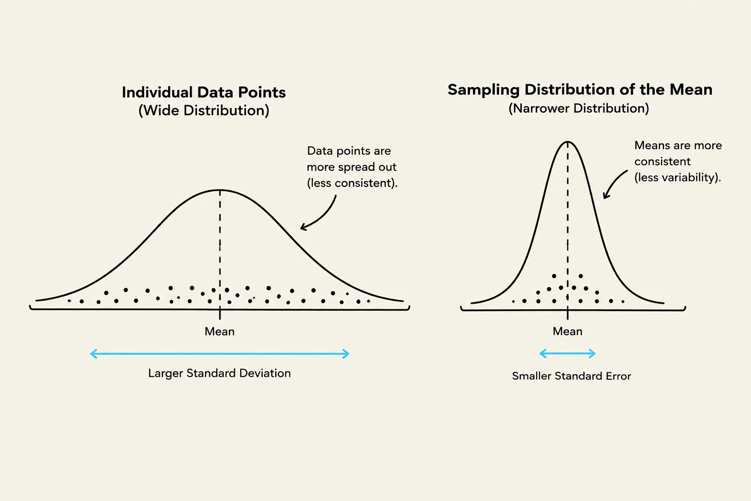
This illustration compares the distribution of individual data points with a wide distribution and a larger standard deviation to the sampling distribution of the mean with a narrower distribution and a smaller standard error, indicating greater consistency.
Step-by-Step Implementation
To conduct a Single-Sample Z Test, follow this structured procedure:
Hypothesis Formulation: State the null hypothesis (H0), which assumes no difference (e.g., μ=μ0), and the alternative hypothesis (Ha).
Two-tailed: Ha states the mean is different from μ0.
One-tailed: Ha states the mean is specifically greater than or less than μ0.
Select your significance level (α), commonly set at 0.05.
Standard Error Calculation: Compute SE=nσ.
Z-score Calculation: Calculate the test statistic (z) to see how many standard errors the sample mean is from the hypothesized mean:
z=SEXˉ−μ0
Probability Determination: Find the p-value (the probability of observing a result as extreme as your test statistic) using a z-table or software.
Decision and Interpretation:
If p≤α, reject H0. The result is statistically significant.
If p>α, do not reject H0.
Worked Example
Suppose a reference population of SAT scores has a mean (μ0) of 511 and a standard deviation (σ) of 120. A researcher tests a sample of 50 students (n=50) who had a mean score (Xˉ) of 535. Using α=0.05:
Step 1: H0:μ=511; Ha:μ=511 (Two-tailed).
Step 2: SE=50120≈16.97.
Step 3: z=16.97535−511≈1.41.
Step 4: For z=1.41 in a two-tailed test, the p-value is approximately 0.16.
Step 5: Since 0.16>0.05, we do not reject H0. There is not enough evidence to say the course changed the scores.
Critical Caution: Statistical significance does not establish a causal relationship. Even if you reject the null hypothesis, the difference might be due to other factors in the research design, and it does not inherently prove "practical importance".
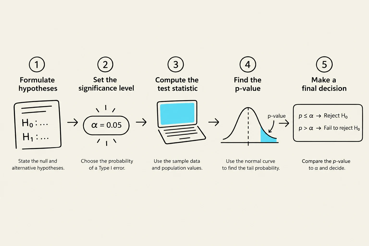
A five-step process for hypothesis testing, including formulating hypotheses, setting the significance level, computing the test statistic, finding the p-value, and making a final decision.
Keep reading for free.
Create an account to finish this reading and make it part of your study routine.