Explore the fundamental concepts of matrix inversion, including transpose, trace, dimensions, and the role of elementary row operations. Learn the inversion algorithm and its connection to solving linear systems.
In linear algebra, finding the inverse of a matrix is a fundamental task that allows us to solve systems of equations of the form $Ax = b$ by calculating x=A−1b. However, not every matrix has an inverse. This article explores the mechanics of matrix inversion, the role of elementary row operations, and the specific algorithm used to transform a matrix into its inverse.
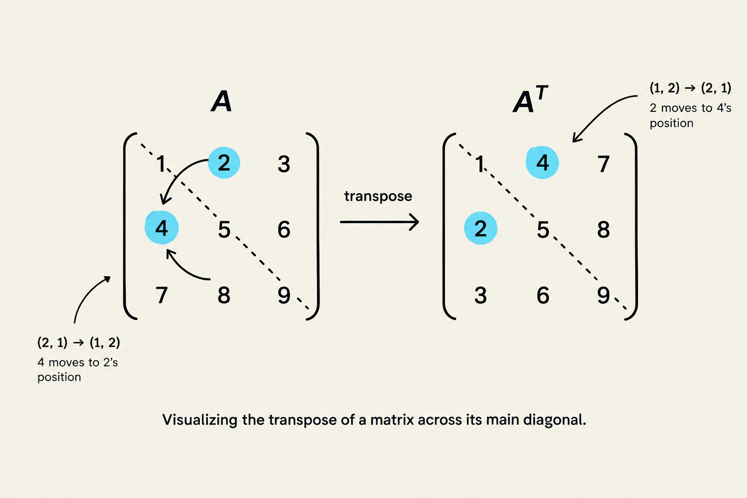
Visualizing the transpose of a matrix across its main diagonal.
Fundamental Matrix Concepts
Before diving into inversion, it is essential to understand the properties of the matrices we are manipulating.
Transpose and Trace of a Matrix
The transpose of a matrix A, denoted as AT, is obtained by interchanging its rows and columns. The relationship between the entries is defined by (AT)ij=(A)ji. For a square matrix, the transpose reflects the entries across the main diagonal, where the diagonal entries themselves remain in their original positions.
The trace of a matrix, denoted as tr(A), is a scalar value representing the sum of the entries on the main diagonal. It is important to note that the trace is only defined for square matrices.
Dimensions and Compatibility
A core habit in matrix algebra is to always check the dimensions of the matrices involved.
Vectors: A matrix can be a row vector (one row) or a column vector (one column).
Multiplication: The product AB is only defined if the number of columns in A matches the number of rows in B.
The Building Blocks: Elementary Matrices and Row Operations
To invert a matrix, we rely on elementary row operations. These operations change the appearance of a matrix without changing the solution set of the underlying linear system. There are three types of operations:
Row Scaling: Multiplying a row by a non-zero constant c (Ri←cRi).
Row Interchange: Swapping two rows (Ri↔Rj).
Row Replacement: Adding a multiple of one row to another (Rj←Rj+cRi).
An elementary matrix is a matrix obtained by performing exactly one of these operations on an identity matrix I. A key theorem in linear algebra states that every elementary matrix is invertible, and its inverse is another elementary matrix that reverses the original operation. For example, if you scale a row by 7, the inverse operation is to scale that same row by 1/7.
The Inversion Algorithm
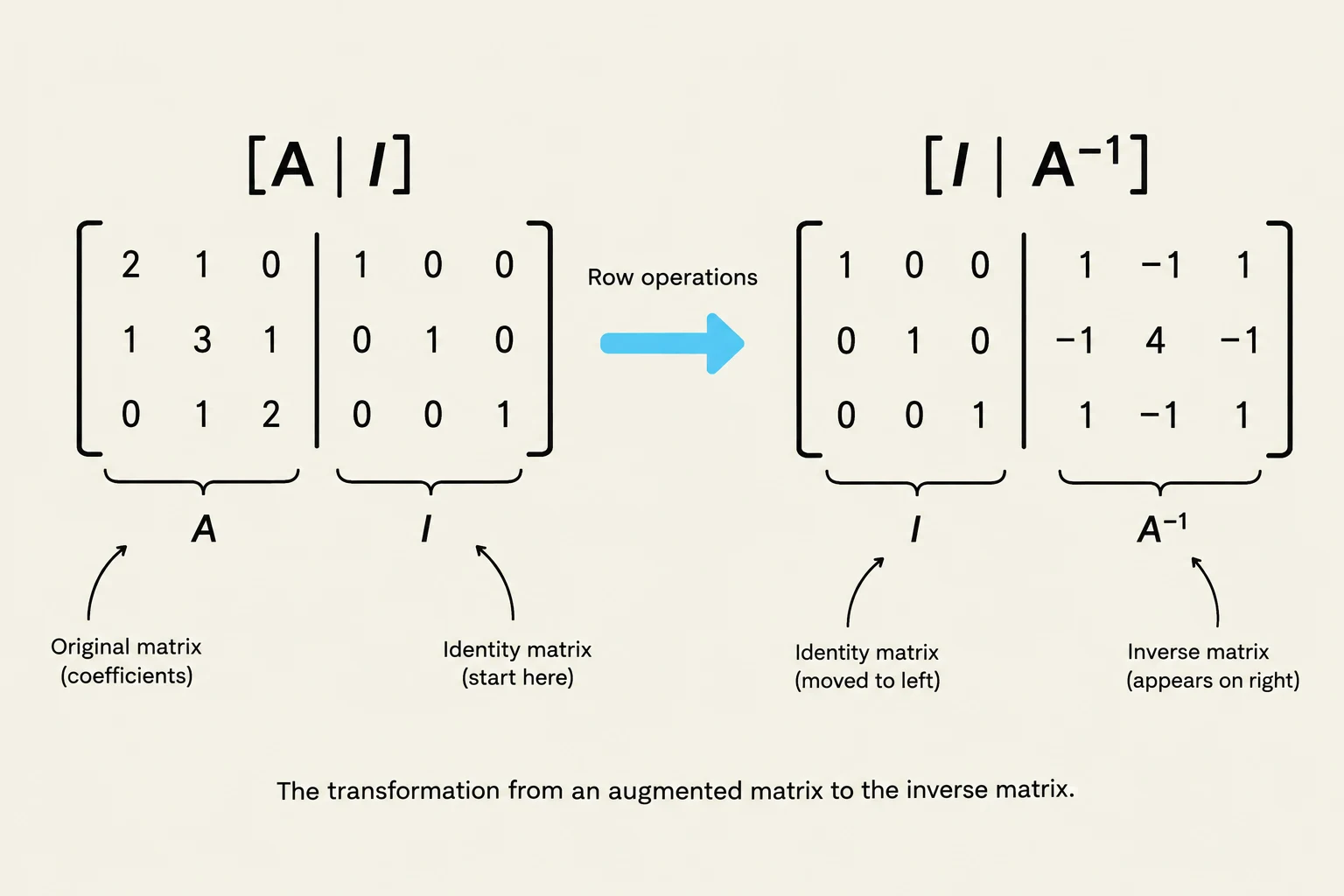
This diagram illustrates the process of finding the inverse of a matrix using row operations. An augmented matrix is formed by combining the original matrix (A) with an identity matrix (I). Through a series of row operations, the identity matrix is transformed into the inverse of the original matrix (A^-1), which appears on the right side of the augmented matrix.
The most common method for finding the inverse of a square matrix A is the Inversion Algorithm. This method utilizes an augmented matrix, which is created by placing the identity matrix I next to A.
The Process
Set up the augmented matrix: Form the block matrix [A∣I].
Row-reduce: Apply elementary row operations to the entire augmented matrix to transform the left side (A) into the identity matrix I.
Extract the result: If you successfully reach the form [I∣A−1], the right side of the partition is your inverse.
Exam Tip: If, during the row-reduction process, you encounter a row of zeros on the left side of the augmented matrix, the matrix A cannot be reduced to I. This means A is noninvertible (also known as a singular matrix).
Worked Example
To find the inverse of A=121250338, we start with the augmented matrix:
121250338100010001
By applying a sequence of row operations (such as R2←R2−2R1 and R3←R3−R1), we eventually transform the left side into I. The resulting matrix on the right is:
A−1=−4013516−5−29−3−1
Invertibility and Linear Systems
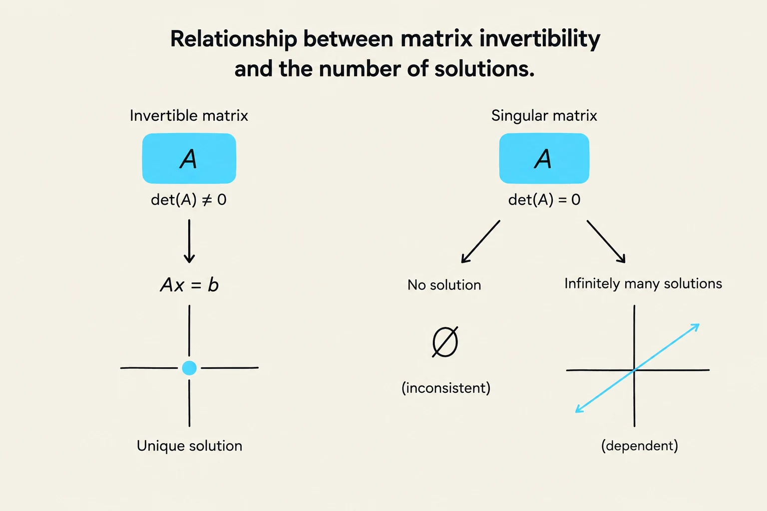
This diagram illustrates the relationship between the invertibility of a matrix and the number of solutions to a system of linear equations represented by Ax = b. An invertible matrix (det(A) ≠ 0) leads to a unique solution. A singular matrix (det(A) = 0) can result in either no solution (inconsistent) or infinitely many solutions (dependent).
The ability to invert a matrix is deeply connected to the nature of the solutions to linear systems. According to the Equivalence Theorem, for an n×n matrix A, the following statements are all equivalent (either all are true or all are false):
A is invertible.
The homogeneous system $Ax = 0$ has only the trivial solution (x=0).
The reduced row echelon form (RREF) of A is the identity matrix In.
A is a product of elementary matrices.
The system $Ax = b$ has exactly one solution for every n×1 matrix b.
If a matrix is singular (noninvertible), the system $Ax = 0$ will have nontrivial solutions (solutions where x=0). In such cases, the system $Ax = b$ might have no solution or infinitely many solutions, depending on the vector b.
Summary Table: Solution Types
Condition
Solution to $Ax = 0$
Solution to $Ax = b$
Invertible Matrix
Only the trivial solution
Exactly one unique solution
Singular Matrix
Nontrivial solutions exist
Zero or infinitely many solutions
Keep reading for free.
Create an account to finish this reading and make it part of your study routine.