Measures of Linear Relationships: Covariance and Correlation
This document explains covariance and correlation as measures of linear relationships between variables. It covers their definitions, formulas for population and sample calculations, and their interpretation, including a worked example.
In statistics, understanding how two different variables interact is fundamental to data analysis. When we observe two sets of data, we often want to know if they move together in a predictable way. This relationship is known as a linear relationship. By using mathematical tools like covariance and correlation, we can quantify whether a change in one variable is associated with a consistent change in another.
Variables and Relationships
Before calculating measures of relationship, we must distinguish between the types of variables involved in a dataset.
Independent and Dependent Variables
In many experimental setups, we distinguish variables based on their role in the relationship:
Independent Variables: These are the variables that are manipulated or controlled to observe an effect.
Dependent Variables: These are the variables that change in response to the independent variable.
For example, in a chemical engineering context, "Catalyst Purity" might be an independent variable used to predict the "Yield of Product," which is the dependent variable.
Linearly Related Random Variables
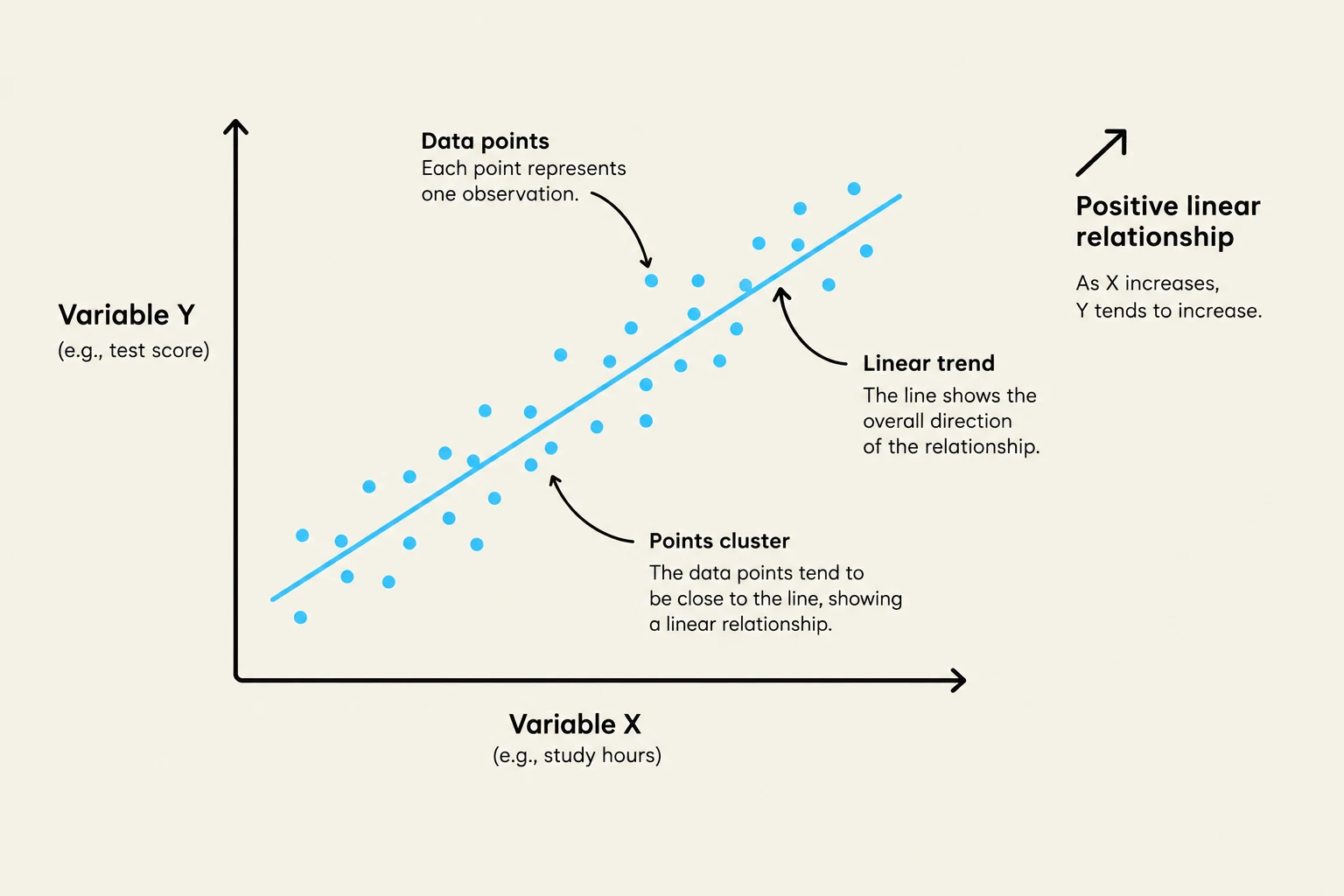
When two random variables exhibit a pattern where they increase or decrease together at a relatively constant rate, they are considered linearly related. If the variables are completely unrelated, they are considered independent. It is important to note that if X and Y are independent random variables, both their covariance and their correlation will be zero.
A scatter plot illustrating a positive linear relationship between two variables, Variable X and Variable Y, with explanations for data points, linear trend, and point clusters.
Understanding Covariance
Covariance is a measure of the linear relationship between two variables. It tells us the direction of the relationship: a positive covariance indicates that the variables tend to move in the same direction, while a negative covariance indicates they move in opposite directions.
The Concept of Variance
To understand covariance, we must first understand variance. Variance (σ2 or Var(X)) is defined as the mean of the squares of the deviations from the mean:
σ2=Var(X)=E[(X−μ)2]=E[X2−2Xμ+μ2]=E[X2]−μ2
Essentially, variance measures how much a single variable spreads out from its own average.
Population vs. Sample Covariance
Depending on whether you are analyzing an entire population or just a subset (a sample), the formula for covariance changes slightly.
1. Population Covariance (σXY):
This is the expected value of the product of the deviations of X and Y from their respective means:
σXY=Cov(X,Y)=E[(X−μX)(Y−μY)]
2. Sample Covariance (sXY):
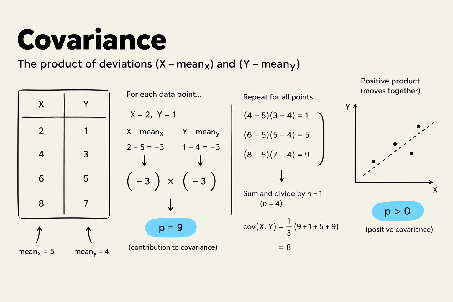
When working with n experimental data points (x1,y1),(x2,y2),…,(xn,yn), we use the sample covariance formula:
sXY=n−11i=1∑n(xi−xˉ)(yi−yˉ)
Note on Units: A major limitation of covariance is that its units are the product of the units of X and Y. For example, if X is measured in centimeters (cm) and Y is in years (yrs), the covariance will be in cm⋅yrs. This makes it difficult to compare the strength of relationships across different types of data.
This illustration explains the concept of covariance, which measures the joint variability of two random variables. It shows how to calculate covariance using a sample dataset by finding the product of deviations from the mean for each data point and then averaging these products. A positive covariance indicates that the variables tend to move in the same direction.
Correlation: The Unitless Measure
Because covariance is tied to the scale of the variables, we use the Correlation Coefficient (ρXY) to compare relationships on a standardized, unitless scale.
The correlation coefficient is calculated by dividing the covariance by the product of the standard deviations of the two variables:
ρXY=σXσYCov(X,Y)
The value of ρXY always falls between −1 and 1:
1: Perfect positive linear relationship.
−1: Perfect negative linear relationship.
0: No linear relationship.
This allows us to compare seemingly incomparable datasets. For instance, comparing the correlation between "Partner Height" and "Partner Age" is impossible using covariance alone because the units (cm2 vs yrs2) differ, but correlation provides a direct comparison.
Worked Example: Calculating Sample Statistics
Let's calculate the sample covariance and sample correlation coefficient for the following datasets:
$X = {5, 2, 4, 3}$
$Y = {3, 6, 4, 5}$
Step 1: Find the means (xˉ and yˉ)
xˉyˉ=45+2+4+3=3.5=43+6+4+5=4.5
Step 2: Calculate the sum of the products of deviations
xi
yi
(xi−xˉ)
(yi−yˉ)
(xi−xˉ)(yi−yˉ)
5
3
1.5
-1.5
-2.25
2
6
-1.5
1.5
-2.25
4
4
0.5
-0.5
-0.25
3
5
-0.5
0.5
-0.25
Total
-5
Step 3: Calculate Sample Covariance (sXY)
sXY=4−11(−5)=3−5≈−1.67
Step 4: Calculate Sample Correlation (rXY)
First, we find the sample variances (sX2 and sY2):
The result rXY=−1 indicates a perfect negative linear relationship between X and Y.
This illustration compares strong positive correlation, where y increases as x increases, with weak correlation, where there is no clear pattern between x and y.
Exam Tip: When asked to compare the "strength" of two relationships, always look at the correlation coefficient (r or ρ), not the covariance. Covariance is sensitive to the scale of the numbers, while correlation is standardized.
Keep reading for free.
Create an account to finish this reading and make it part of your study routine.