Measures of Dispersion and Variability in Statistics
Learn about statistical dispersion, which measures how spread out data points are. This guide covers basic measures like range and extremes, and more advanced concepts like variance, standard deviation, and the coefficient of variation.
When analyzing data, knowing the "average" value is often not enough. For example, if you are looking at the annual salaries of employees in two different companies, both might have an average salary of £50,000. However, in one company, everyone might earn between £45,000 and £55,000, while in the other, some earn £20,000 and others earn £150,000. To understand this difference, we need to look beyond the center of the data and examine its spread. This is the role of statistical dispersion.
Understanding Statistical Dispersion
Statistical dispersion refers to how "spread out" or scattered the observations in a data series are. While measures of location (like the arithmetic mean, median, and mode) tell us where the center of the data lies, measures of dispersion tell us how much the individual data points deviate from that center.
A high level of dispersion indicates that the data points are far from the mean and from each other, suggesting high variability. Conversely, low dispersion indicates that the data points tend to be very close to the mean and to each other.
Basic Measures: Range and Extremes
The simplest way to begin assessing dispersion is by looking at the boundaries of your dataset: the minimum and maximum values. These extreme values provide a first indication of the data's spread and can be particularly useful for detecting "unusual" values or potential data entry errors.
From these two values, we can calculate the range, which is the total difference between the maximum and the minimum values in the series.
Note: While the range is easy to calculate, it is highly sensitive to outliers. A single extremely high or low value can significantly inflate the range, potentially giving a misleading impression of the typical spread of the data.
Variance and Standard Deviation
To get a more sophisticated understanding of variability, we use variance, which measures the average squared distance between each observation and the arithmetic mean. Because we square the differences, variance is always a positive number, and it heavily penalizes observations that are far from the mean.
Depending on whether you are analyzing an entire group or just a subset, you will use one of two formulas:
Population Variance
If you have data for every single member of the group you are studying (the population), you calculate the population variance (σ2) as follows:
σ2=N∑i=1N(xi−μ)2
Where:
μ is the population mean.
N is the population size.
xi is the ith value in the population.
Sample Variance
In most real-world scenarios, we only have access to a subset of the population (a sample). To account for the fact that a sample is only an estimate, we use the sample variance (s2), which uses n−1 in the denominator instead of n:
s2=n−1∑i=1n(xi−xˉ)2
Where:
xˉ is the sample arithmetic mean.
n is the sample size.
Standard Deviation
While variance is mathematically useful, it can be difficult to interpret because its units are squared (e.g., if you are measuring height in meters, variance is in "meters squared"). To solve this, we use the standard deviation (s or σ), which is simply the square root of the variance:
Standard Deviation=Variance
The standard deviation is the most commonly used measure of variability because it returns the measurement to the same units as the original data, making it much easier to interpret.
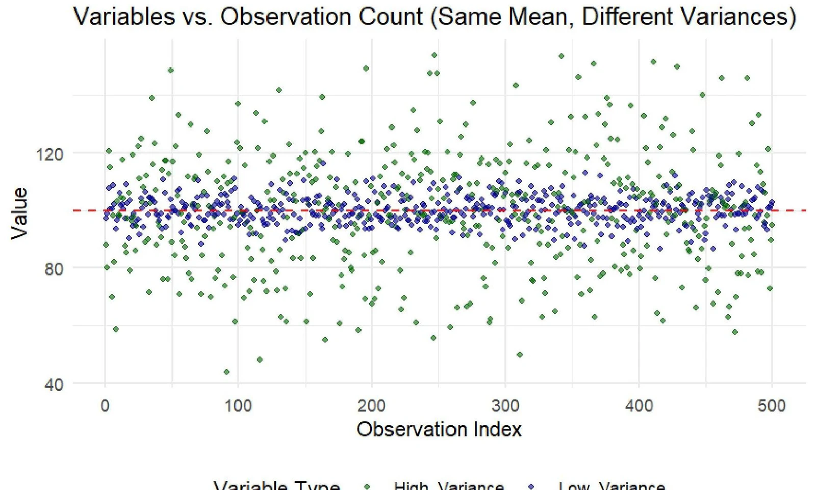
This scatter plot illustrates two variables with the same mean but different variances. The x-axis represents the observation index, and the y-axis represents the value. The plot shows that the 'High Variance' variable (green dots) has a wider spread of values compared to the 'Low Variance' variable (blue dots), which is clustered more closely around the mean (indicated by the dashed red line).Figure 1: Visualizing how different standard deviations affect data spread even when the mean is identical.
The Coefficient of Variation (CoV)
A common question in statistics is: "Is this standard deviation high or low?" The answer depends on the scale of the data. A standard deviation of £100 is massive if you are measuring the price of a loaf of bread, but it is negligible if you are measuring the price of a luxury car.
To compare variability across different datasets or different units, we use the Coefficient of Variation (CoV). This is a measure of relative consistency that expresses the standard deviation as a proportion of the arithmetic mean:
Coefficient of Variation=Arithmetic MeanStandard Deviation
High CoV (e.g., > 1): Suggests the data is widely dispersed relative to the mean. In such cases, the arithmetic mean might not be a representative "typical" value for the dataset.
Low CoV: Suggests the data is more consistent and clustered closely around the mean.
Exam Tip: Remember that a high or low CoV is not inherently "good" or "bad"; it is simply a descriptive feature of the data. However, if you are using the mean to create a forecast, a high CoV serves as a warning that your forecast may be unreliable.
Keep reading for free.
Create an account to finish this reading and make it part of your study routine.