Explore the fundamental concepts of linear equations and systems, including their definitions, classifications of solutions (unique, infinite, none), and geometric interpretations. Learn about homogeneous and non-homogeneous equations, and the role of unknowns and ordered n-tuples in representing solutions.
In the study of linear algebra, the most fundamental building block is the linear equation. While a single equation might seem simple, combining multiple equations into a "system" allows us to model complex relationships in science, engineering, and economics. Understanding how to identify these equations, solve their systems, and interpret their solutions geometrically is essential for everything that follows in the course.
The Linear Equation
This illustration differentiates between linear and non-linear equations by showing examples of each and their corresponding graphical representations.
A linear equation is an algebraic equation where the variables are raised only to the first power and are combined with constant coefficients. The general form for an equation with n variables is:
a1x1+a2x2+⋯+anxn=b
In this expression, a1,a2,…,an are constants.
Special Cases and Recognition
Depending on the value of the constant b, we can classify the equation further:
Homogeneous Linear Equation: If b=0, the equation is called homogeneous.
Non-homogeneous: If b=0, it is non-homogeneous.
To ensure an equation remains linear, you must watch out for "rule-breakers." An equation is not linear if it contains:
Variable products (e.g., $xy = 5$).
Roots (e.g., x=2).
Powers other than 1 (e.g., x2+y=4).
Variables inside trigonometric, logarithmic, or exponential functions (e.g., sin(x)=0).
Systems, Unknowns, and Solutions
A linear system is a finite set of one or more linear equations involving the same set of variables. The variables within these equations are referred to as unknowns.
A solution to a system is a set of values that makes every single equation in that system true simultaneously. Because the order of variables matters, we express a solution as an ordered n-tuple:
(s1,s2,…,sn)
For example, in a system with two unknowns x and y, a solution might be written as (1,−2), where x=1 and y=−2.
Classification of Solutions
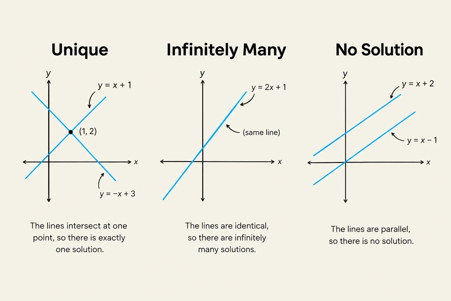
This illustration shows three scenarios for systems of linear equations: unique solution (intersecting lines), infinitely many solutions (identical lines), and no solution (parallel lines).
One of the most important concepts in linear algebra is that every linear system falls into exactly one of three categories regarding its solution set:
1. Consistent Systems
A system is consistent if it has at least one solution. Consistent systems are further divided into two types:
Unique Solution (One Solution): The system has exactly one specific value for each unknown.
Geometric Meaning: In two dimensions, this represents two lines intersecting at a single point. In three dimensions, it represents three planes meeting at a single point.
Infinitely Many Solutions: This occurs when the equations are redundant, meaning they don't provide enough unique information to pin down a single point.
Geometric Meaning: This represents lines or planes that overlap or intersect along a line or a plane.
Free Parameters: To describe these solutions, we use parameters (often denoted as $t, r,$ or s). For example, if y can be anything, we might set y=t and express x in terms of t.
2. Inconsistent Systems
A system is inconsistent if it has no solution. This happens when the equations contradict each other (for example, if simplification leads to a statement like 0=−6).
Geometric Meaning: In two dimensions, this represents parallel and distinct lines. In three dimensions, it represents planes that have no common intersection point.
Exam Tip: When solving a system, if you reach a row that looks like 0=non-zero number, stop immediately! The system is inconsistent and has no solution.
Solving Systems: Elimination and Matrices
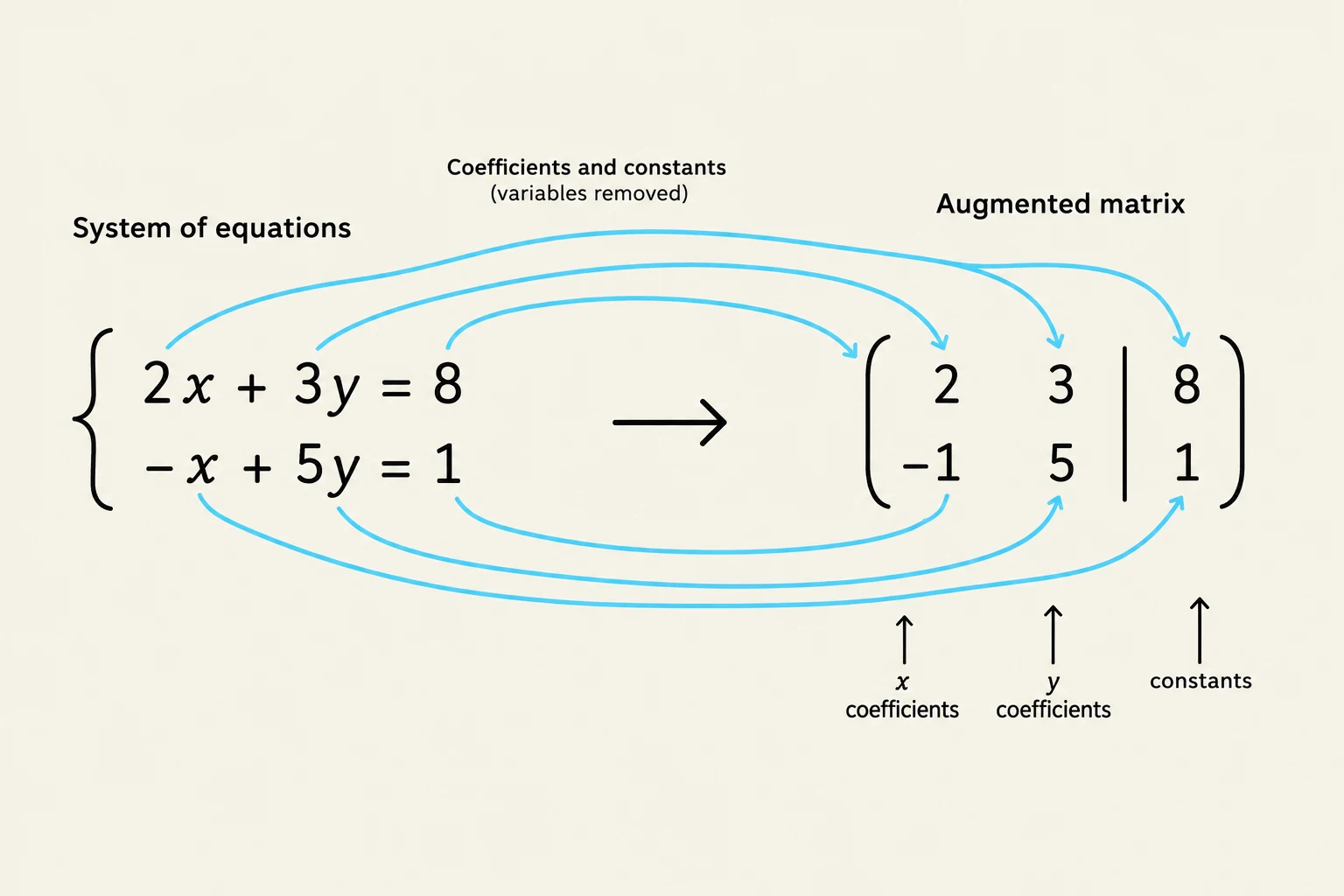
This illustration demonstrates how a system of linear equations can be represented as an augmented matrix, which is a common technique in linear algebra.
To find these solutions systematically, we use the method of elimination. While we can do this with standard algebra, it is more efficient to use an augmented matrix, which strips away the variable symbols and keeps only the coefficients and constants.
Elementary Row Operations
To solve an augmented matrix, we use three specific operations that change the appearance of the matrix without changing the solution set of the system:
Scale: Multiply a row by any nonzero constant (Ri→cRi).
Swap: Interchange two rows (Ri↔Rj).
Replace: Add a multiple of one row to another (Rj→Rj+cRi).
By applying these operations, we aim to reach a "triangular" form or a reduced form where the solutions become obvious.
Result of Row Reduction
Solution Type
A pivot in every variable column
Unique Solution
A row like $[0 \dots 0
\text{non-zero}]$
No Solution |
| A row like [0…0∣0] (with free variables) | Infinitely Many Solutions |
Keep reading for free.
Create an account to finish this reading and make it part of your study routine.