This guide explains the fundamental concepts of statistical hypothesis testing, including developing null and alternative hypotheses, understanding Type I and Type II errors, and interpreting p-values. It covers one-tailed and two-tailed tests, as well as methods for comparing two populations and measuring effect size.
In a world filled with misinformation and conspiracy theories, statistical testing serves as a vital tool for "myth busting". Whether a business is testing a new marketing claim, an economist is evaluating the Law of Demand, or a scientist is verifying a medical theory, hypothesis testing provides a formal, mathematical framework to move beyond intuition and into evidence-based decision-making.
At its core, hypothesis testing is a procedure used to evaluate claims about a population mean (μ) by analyzing sample data. By using samples, we can make inferences about much larger groups, helping us predict future outcomes and validate theories.
Developing Hypotheses: The Null and Alternative
A hypothesis is a tentative statement or prediction regarding the results of a research study. In formal testing, we do not just test one idea; we test two mutually exclusive and opposite statements.
The Null Hypothesis (H0)
The Null Hypothesis is the tentative assumption or the claim that is assumed to be true at the start of the test. It often represents the status quo, or the idea that there is "no effect" or "no difference". For example, if a company claims a drink provides 5 hours of energy, the null hypothesis would be that the energy boost is at least 5 hours (H0:μ≥5).
The Alternative Hypothesis (Ha or H1)
The Alternative Hypothesis is the counter-claim that a researcher seeks to support. It is the statement that contradicts the null hypothesis. If the researcher finds sufficient evidence that the energy boost is actually less than 5 hours, they would support the alternative hypothesis (H1:μ<5).
The relationship between these two is mathematically strict: if H0 contains equality ($=$, ≥, or ≤), then Ha must contain inequality (=, $<$, or $>$), and vice versa.
Directional vs. Non-Directional Tests
Hypotheses are categorized based on whether the researcher is looking for a difference in a specific direction or just any difference at all.
One-Tailed Hypotheses
One-tailed tests are used when the alternative hypothesis points in a single direction—either "greater than" or "less than".
Lower Tail: Used when the researcher suspects the parameter is less than a certain value.
H0:μ≥value
H1:μ<value
Upper Tail: Used when the researcher suspects the parameter is greater than a certain value.
H0:μ≤value
H1:μ>value
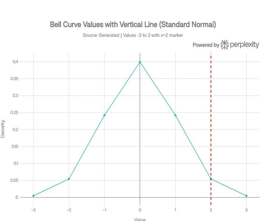
A bell curve illustrating the standard normal distribution with a vertical line at x=2.
Two-Tailed Hypotheses
Two-tailed tests are used when the researcher wants to test for any difference, regardless of direction. This is often used in "is/is not" or "equal/not equal" scenarios. For example, if a snack box claims to have exactly 100 calories, a two-tailed test would check if the actual mean is simply not equal to 100.
H0:μ=value
H1:μ=value
Understanding Errors in Decision Making
Because we are using samples to make guesses about entire populations, there is always a risk of making the wrong conclusion. These mistakes are categorized as Type I and Type II errors.
Decision
H0 is True
H0 is False (Ha is True)
Reject H0
Type I Error (α)
Accurate (Correct Decision)
Accept H0
Accurate (Correct Decision)
Type II Error (β)
Type I Error
A Type I Error occurs when we reject the null hypothesis even though it is actually true. This is often linked to the significance level (α). A classic example is a medical test telling a person they are pregnant when they are actually not.
Type II Error
A Type II Error occurs when we accept (fail to reject) the null hypothesis even though it is actually false. This is a "false negative"—failing to find a symptom or effect that actually exists. An example would be a doctor telling a visibly pregnant woman that she is not pregnant.
Exam Tip: Remember that Type I is a "False Positive" (claiming something happened when it didn't) and Type II is a "False Negative" (claiming nothing happened when it actually did).
The P-Value: Measuring Evidence
The p-value is the probability of obtaining a test statistic at least as extreme as the one observed, assuming the null hypothesis is true. It tells us how "surprising" our sample data is.
Small p-value (≤α): The result is highly significant. We reject the null hypothesis.
Large p-value (>α): The result is not statistically significant. We fail to reject (accept) the null hypothesis.
This diagram illustrates the relationship between statistical significance levels and the strength of evidence. Lower p-values (closer to 0) indicate stronger evidence, while higher p-values suggest weaker or no evidence.
Testing Two Populations
Sometimes, we aren't just testing one group; we want to compare two different populations, such as comparing the stock values of Alphabet vs. Apple or the GPA of freshmen vs. seniors.
Independent Samples
When two samples are collected separately and independently from two distinct populations, they are called Independent Simple Random Samples. To test the difference between their means (μ1−μ2), we use the difference between their sample means (Xˉ1−Xˉ2) as our point estimator.
When performing a t-test for two populations where the variance (σ) is unknown, we must consider the data's spread:
Equal Variance: The data spreads in a similar pattern across both samples.
Unequal Variance: One sample shows a significantly wider or different spread than the other.
Matched (Paired) Samples
In other cases, the samples are not independent. A Matched Sample occurs when each sampled item provides a pair of data values. A common example is a "Pre-Test" and "Post-Test" design, such as measuring a pet's weight before and after a diet intervention. Because the data points are linked, matched samples typically result in a smaller sampling error than independent designs.
Measuring Effect Size
Even if we reject the null hypothesis, we must ask: How much does it matter? This is where Effect Size comes in. Using Cohen's d, we can categorize the magnitude of the difference between two means:
d=spooledxˉ1−xˉ2
Small Effect:d≈0.2
Medium Effect:d≈0.5
Large Effect:d≈0.8+
By combining hypothesis testing with effect size, researchers can determine not only if a result is statistically significant but also if it is practically meaningful in the real world.
Keep reading for free.
Create an account to finish this reading and make it part of your study routine.