Statistics is much more than a collection of mere numbers and figures; it is a comprehensive set of techniques and procedures used for analyzing, interpreting, displaying, and making decisions based on data. Whether we are looking at the percentage of birth certificates issued in a specific state or the average winning time in an Olympic marathon, statistics allow us to find patterns and meaning in a sea of information. To master statistics, one must first understand the fundamental building blocks: how we define variables, how we measure them, and how we organize those measurements into distributions.
The Two Branches of Statistics
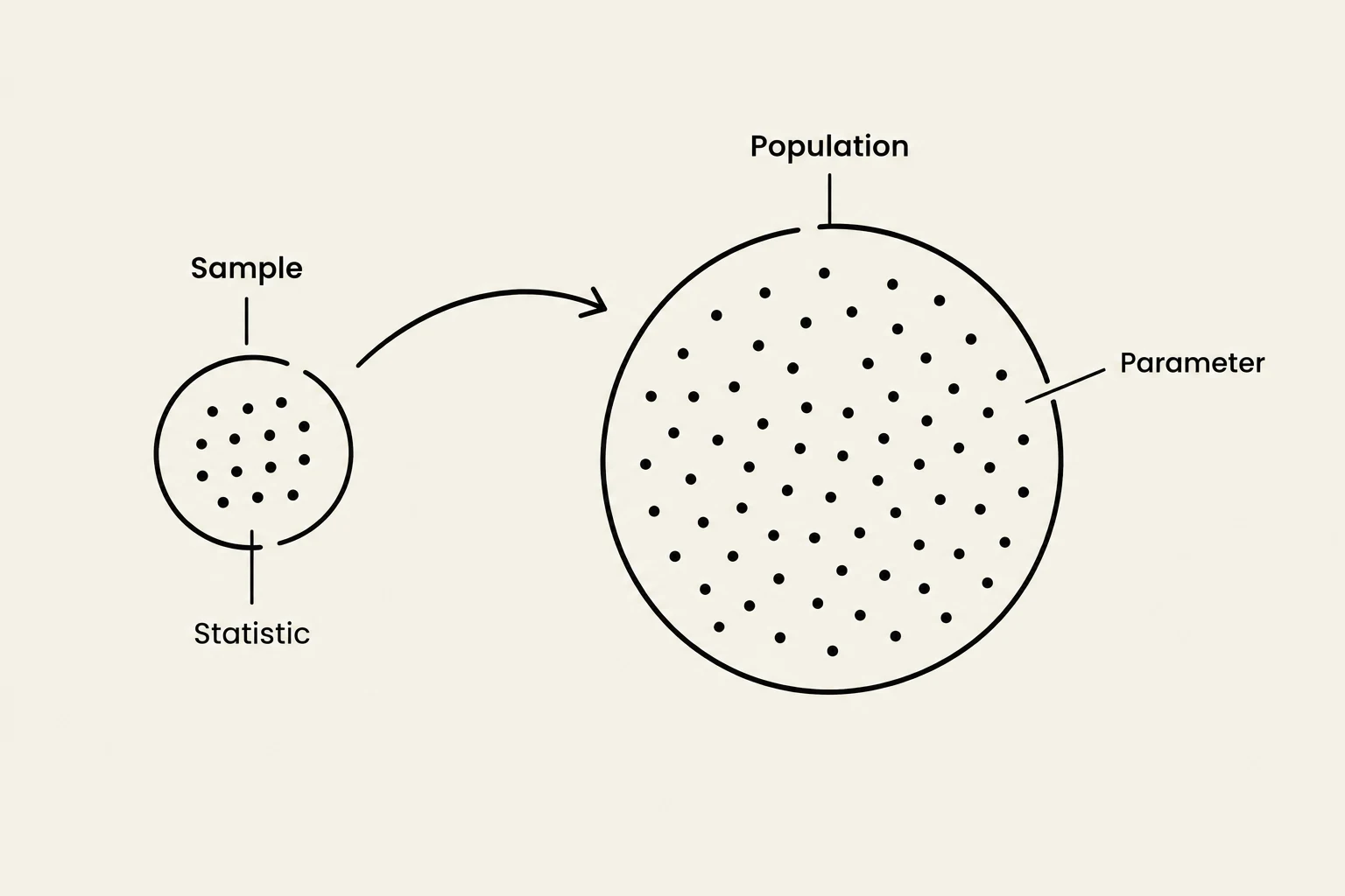
This diagram illustrates the relationship between a sample and a population in statistics. A sample is a subset of a population, and a statistic is a measure calculated from a sample, which is used to estimate a parameter of the population.
The field of statistics is broadly divided into two primary domains: descriptive and inferential statistics.
Descriptive statistics are used to summarize and describe the characteristics of a specific set of data. They provide a "snapshot" of the data at hand—such as the average salary of an occupation or the number of unmarried men in a specific city—without attempting to make claims about anyone outside that specific group.
Inferential statistics, on the other hand, involve drawing conclusions about a population based on a sample.
A population is the complete set of observations for a well-defined group (e.g., every college senior in the United States).
A sample is a subset of that population (e.g., 500 students selected from various universities).
Because it is often impossible or prohibitively expensive to measure every member of a population, we use the sample to make "intelligent guesses" about the whole. When we calculate a value for a population (like a population mean), we call it a parameter. When we calculate a value from a sample, we call it a statistic.
Exam Tip: Remember the distinction between Parameter and Statistic. Parameter goes with Population; Statistic goes with Sample.
Understanding Variables
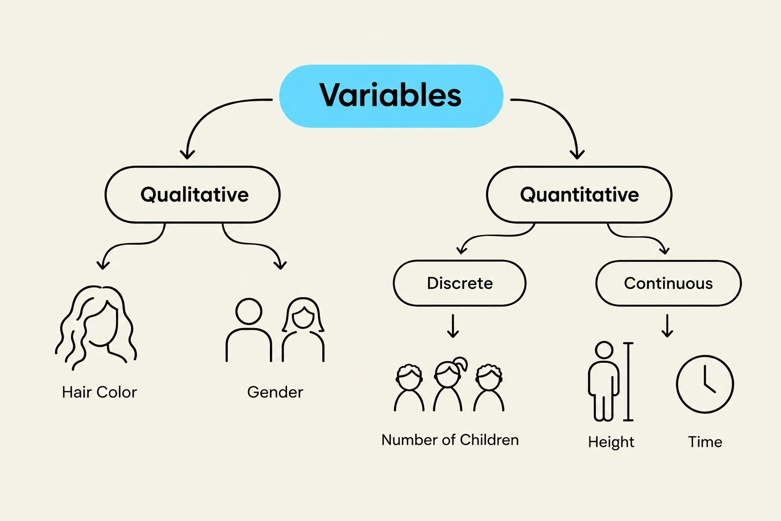
This diagram illustrates the classification of variables into qualitative and quantitative types, with further subcategories for discrete and continuous quantitative variables.
A variable is any characteristic that can take on different values. In research, we often look at how one variable affects another. The variable manipulated by the researcher is the independent variable, while the variable being measured to see the effect is the dependent variable.
Variables are categorized by their nature and the way they are measured:
Qualitative vs. Quantitative
Qualitative variables (also called categorical variables) express attributes that have no natural sense of numerical ordering, such as hair color, religion, or gender.
Quantitative variables are measured on a numeric scale, such as height, weight, or test scores.
Discrete vs. Continuous
Discrete variables take on a limited and fixed number of values or distinct categories. For example, the number of children in a household is discrete; you can have 2 or 3 children, but not 2.45.
Continuous variables can take on any value between two specified points. An example is "time to respond to a question," which could be 1.64 seconds or 1.64237 seconds.
Organizing Data: Distributions
A distribution is the collection of all scores for a specific variable. To make sense of these scores, we organize them into various formats.
Frequency Distributions and Tables
A frequency distribution (or frequency table) is a listing of unique scores and the number of times each score occurs in a distribution. To further analyze these, we use:
Relative frequency: The proportion of scores falling into various classes.
Cumulative frequency: The running total of scores displayed for a set of unique values, listed from low to high.
Continuous Distributions and Probability
When dealing with continuous variables, we often use a grouped frequency distribution to tabulate scores within specific ranges, which can be visualized using a histogram.
In more advanced contexts, we look at a probability distribution, which describes the proportions of scores across an entire population. For continuous variables, we refer to this as a continuous distribution. In a normal distribution (a symmetric, bell-shaped curve), the total area under the curve equals 1. This means the probability of any single, exact value occurring is 0, but the area between two points represents the probability of a value falling within that specific range.
The Shape of Distributions
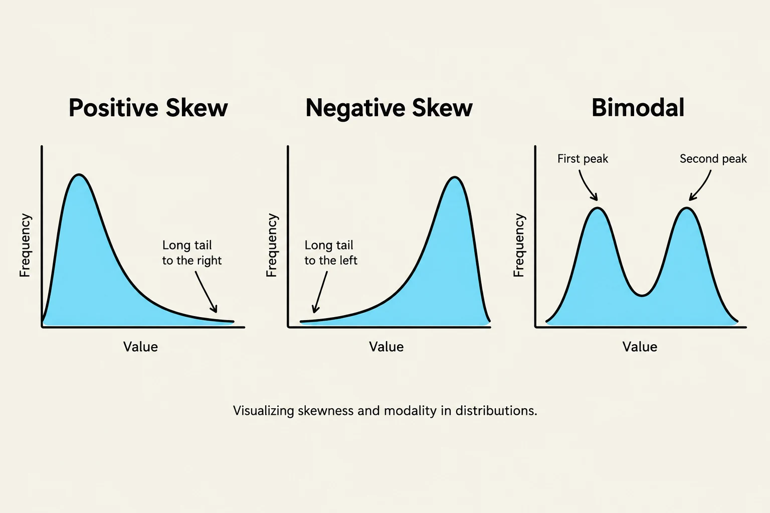
Visualizing skewness and modality in distributions.
The "shape" of a distribution tells us a lot about the data. We classify shapes using three main concepts:
1. Skewness (The Tail)
Skewness refers to the direction in which the "tail" of the distribution extends.
Positive Skew (Skewed Right): The tail extends toward the higher (positive) values. An example is professional athlete salaries, where most players earn modest amounts, but a few superstars earn massive amounts, pulling the tail to the right.
Negative Skew (Skewed Left): The tail extends toward the lower (negative) values.
2. Modality (The Peaks)
Modality refers to the number of peaks in a distribution.
A bimodal distribution has two distinct peaks. An example is the frequency of eruption times for the Old Faithful geyser, which shows two distinct peaks.
3. Kurtosis (The Tails)
Kurtosis describes the thickness or "fatness" of the tails.
Leptokurtic: A distribution with relatively fat or long tails.
Platykurtic: A distribution with relatively thin or short tails.
Percentiles: Where Do You Stand?
A single score (like a 35/50 on a test) is hard to interpret without context. Percentiles provide that context by showing your position relative to others.
Percentile Rank: The proportion of scores that fall at or below a particular score value. If you are in the 65th percentile, 65% of people scored at or below you.
Percentile Score: The specific score in a distribution that represents a certain percentile.
Edge Case Alert: There is no single universal definition for calculating percentiles. Some definitions use "greater than" while others use "greater than or equal to." In most textbooks, a weighted average (interpolation) is used to handle these differences more gracefully.
Mathematical Tools: Summation Notation
In statistics, we frequently need to add long series of numbers. To avoid writing out every single value, we use summation notation. The Greek letter Σ (sigma) is the symbol for summation.
For a set of values X1,X2,X3,X4, the sum is written as:
∑i=14Xi
If we want to sum all values of X without specifying a range, we use the abbreviated notation:
∑X
It is vital to distinguish between summing a square and squaring a sum:
∑X2 means you square each number first, then add them up.
(∑X)2 means you add all the numbers first, then square the total.
Measurement and Validity
To ensure our data is useful, we must consider the quality of our measurement. Measurement is the process of assigning numbers to characteristics based on specific rules.
Validity
Validity refers to the extent to which a measurement represents what it is intended to measure.
Face Validity: Does the test appear to measure what it is supposed to at first glance?
Construct Validity: To what extent do the values of one measure correlate with another measure that is presumed to measure the same thing?
Reliability
While validity is about accuracy, reliability is about consistency. A reliable measurement will yield the same results repeatedly under the same conditions.
Summary Note: A measurement can be reliable (consistent) without being valid (accurate), but it cannot be truly valid if it is not reliable.
Keep reading for free.
Create an account to finish this reading and make it part of your study routine.