Introduction to Simple Linear Regression in Econometrics
This guide explains the fundamental concepts of the simple linear regression model, including its mathematical formulation, the role of the error term, Ordinary Least Squares (OLS) estimation, and methods for measuring goodness of fit like R-squared.
Econometrics allows us to move beyond simple observation to quantify the relationships between different economic phenomena. At the heart of this discipline lies the Simple Linear Regression model, a tool used to estimate how much a change in one variable affects another. Whether we are studying how years of education impact hourly wages or how income influences consumption, simple linear regression provides the mathematical foundation for these inquiries.
The Simple Linear Regression Model
The most basic econometric model is expressed by the following equation:
y=β1+β2x+e
In this model, we distinguish between two primary types of variables:
The Dependent Variable (y): Also known as the explained variable, response, or regressand. This is the outcome we are trying to understand or predict.
The Independent Variable (x): Also known as the explanatory variable, control, or regressor. This is the factor we believe influences y.
The relationship is governed by two parameters: β1, which represents the intercept (the value of y when x=0), and β2, which represents the slope (the change in y for a one-unit change in x).
The Role of the Error Term
No mathematical model can perfectly capture the complexity of the real world. Therefore, we include an error term (e), often called the "disturbance". You can think of the error term as a "trash can" that collects all the unobserved factors that affect y but are not explicitly included in our model. For example, in a model predicting wages based on education, the error term might contain unobserved factors like innate ability, work ethic, or sheer luck.
For our estimate of the slope (β2) to be unbiased, we must assume that the independent variable x is uncorrelated with this error term, expressed as Corr(x,e)=0.
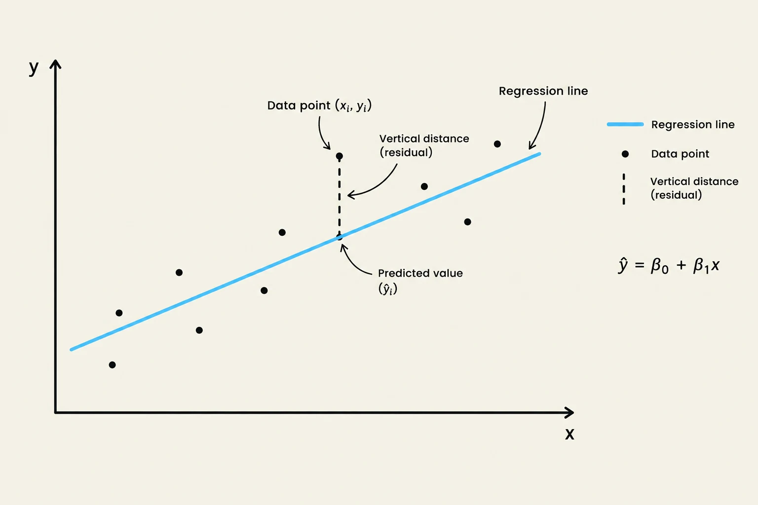
This graph illustrates a linear regression model, showing data points, a regression line, and the concept of residuals (vertical distances between data points and the regression line).
Ordinary Least Squares (OLS) Estimation
To make sense of our data, we need to estimate the values of β1 and β2. The standard method used in econometrics is Ordinary Least Squares (OLS).
The goal of OLS is to find the "best-fit" line by minimizing the sum of squared residuals. A residual (e^i) is the difference between the actual observed value (yi) and the value predicted by our model (y^i), where y^i=β^1+β^2xi. The minimization formula is:
β^1,β^2mini=1∑n(yi−y^i)2
Why Square the Residuals?
You might wonder why we don't simply minimize the sum of the residuals. There are two main reasons:
Cancellation: If we just summed the residuals, positive and negative errors would cancel each other out, potentially resulting in a sum of zero even if the line fits the data very poorly.
Mathematical Convenience: Squaring the errors penalizes large outliers more heavily and makes the function much easier to differentiate when solving for the minimum.
Measuring Goodness of Fit
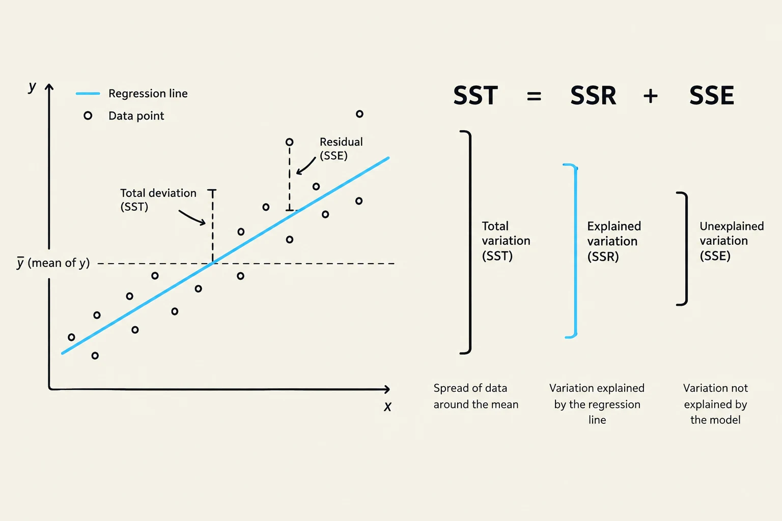
Once we have estimated our line, we need to know how well it actually describes the data. To do this, we decompose the total variation in y into three distinct components:
Total Sum of Squares (SST): The total variation in the observed y values around their mean (yˉ), calculated as ∑(yi−yˉ)2.
Explained Sum of Squares (SSE): The portion of the variation that is explained by our regressor x, calculated as ∑(y^i−yˉ)2.
Residual Sum of Squares (SSR): The portion of the variation that remains unexplained by the model, calculated as ∑e^i2.
These components are related by the identity: $SST = SSE + SSR$.
The R2 Coefficient
The most common way to express "goodness of fit" is through R2 (R-squared). This value represents the proportion of the total variation in y that is explained by x:
R2=SSTSSE=1−SSTSSR
The value of R2 always falls between 0 and 1. An R2 of 0.80, for instance, means that 80% of the variation in the dependent variable is explained by the model.
Exam Tip: A high R2 does not prove causation. A high R2 only indicates that there is a strong correlation or "fit" between the variables. Causal inference depends on the underlying assumptions of the model, such as the absence of omitted variable bias.
This diagram illustrates the concept of total sum of squares (SST) in regression analysis, which is decomposed into the sum of squares due to regression (SSR) and the sum of squares due to error (SSE).
Linearity in Parameters
A common point of confusion is what "linear" actually means in "Simple Linear Regression." In econometrics, "linear" refers to the model being linear in parameters (βs).
This is a very flexible property. It means that while the β coefficients must appear in a linear form, the variables themselves (x or y) can be transformed in non-linear ways, such as using logarithms.
Common Functional Forms
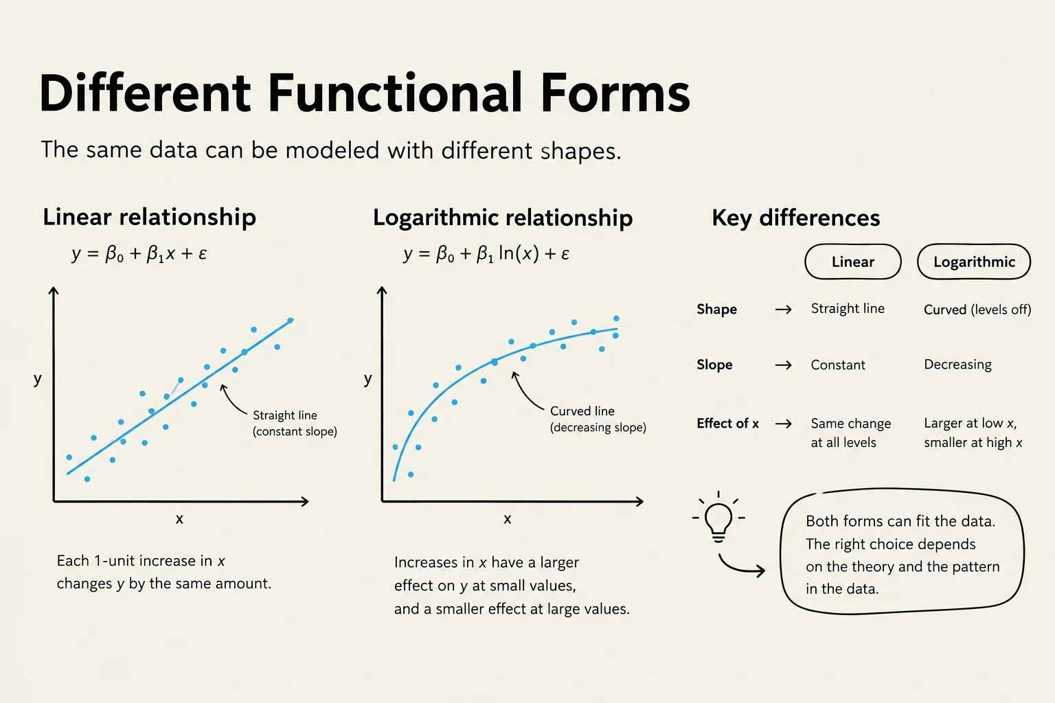
By using logarithms, we can model various types of relationships and interpret the results in terms of percentages:
Level-Level (Lin-Lin):y=β1+β2x. A 1-unit change in x leads to a β2 unit change in y.
Log-Level (Log-Lin):ln(y)=β1+β2x. A 1-unit change in x leads to an approximate (100⋅β2)% change in y.
Level-Log (Lin-Log):y=β1+β2ln(x). A 1% change in x leads to an approximate (β2/100) unit change in y.
Log-Log (Constant Elasticity):ln(y)=β1+β2ln(x). A 1% change in x leads to a β2% change in y. Here, β2 is known as the elasticity.
This illustration compares linear and logarithmic functional forms, showing their graphical representations, mathematical equations, and key differences in shape, slope, and the effect of x on y. It also notes that the choice of model depends on the data and theory.
Summary Table of Interpretations
Model Type
Equation
Interpretation of β2
Common Name
Lin-Lin
y=β1+β2x
Δx=1⟹Δy=β2
Slope
Log-Lin
ln(y)=β1+β2x
Δx=1⟹Δy≈100β2%
Semi-Elasticity
Lin-Log
y=β1+β2ln(x)
Δx=1%⟹Δy≈β2/100
Semi-Elasticity
Log-Log
ln(y)=β1+β2ln(x)
Δx=1%⟹Δy≈β2%
Elasticity
Keep reading for free.
Create an account to finish this reading and make it part of your study routine.