Introduction to Rectilinear Kinematics and Erratic Motion
Explore the fundamental concepts of rectilinear kinematics, including position, displacement, velocity, and acceleration. Learn how calculus is applied to analyze motion and understand erratic motion through graphical methods.
In the study of dynamics, we distinguish between kinetics—the study of forces—and kinematics, which focuses purely on the geometric aspects of motion. When a particle moves along a straight line, we refer to this as rectilinear kinematics. Understanding how to describe this motion is fundamental to engineering, whether you are analyzing the trajectory of a projectile or the acceleration of a vehicle.
Fundamental Kinematic Quantities
To describe rectilinear motion, we must define three primary variables: position, velocity, and acceleration.
Position and Displacement
The position of a particle is defined using a single coordinate axis s with a fixed origin O. The position s is a vector quantity, though it is often represented by a scalar value where the sign indicates the direction relative to the origin.
Displacement, denoted as Δs, is the change in position:
Δs=s′−s
It is important to distinguish displacement from distance. While displacement is a vector representing the change in position, distance is a positive scalar representing the total path length traveled.
Instantaneous Velocity and Speed
Average velocity is the displacement divided by the time interval: vavg=Δs/Δt. However, in most engineering applications, we require the instantaneous velocity, which is the limit as the time interval approaches zero:
v=dtds
The magnitude of this velocity is known as the speed.
Instantaneous Acceleration
Acceleration describes how the velocity changes over time. The instantaneous acceleration a is defined as:
a=dtdv=dt2d2s
If a particle's speed is decreasing, it is said to be decelerating.
Exam Tip: A particle can have zero velocity but still possess acceleration. For example, a ball thrown vertically upward has zero velocity at its highest point, but its acceleration is still 9.81 m/s2 downward.
Calculus in Kinematics: Differentiation and Integration
The relationships between s, v, and a are governed by differential calculus. By using differentiation, we can move from position to velocity, and from velocity to acceleration. Conversely, by using integration, we can move from acceleration to velocity, or from velocity to position.
A vital relationship used when time is not explicitly involved is obtained by eliminating the time differential dt from the definitions of v and a:
dt=vds=adv
Which leads to the useful identity:
$a , ds = v , dv$
Constant Acceleration
When acceleration is constant (a=ac), we can use integrated formulas to relate the variables directly:
Velocity vs. Time:v=v0+act
Position vs. Time:s=s0+v0t+21act2
Velocity vs. Position:v2=v02+2ac(s−s0)
Erratic Motion and Graphical Analysis
In many real-world scenarios, acceleration is not constant; this is known as erratic motion. In these cases, we cannot use the simplified constant acceleration formulas and must rely on calculus to solve for unknowns.
To visualize and solve these complex motions, we use several types of graphs:
Time-Based Graphs ($s-t, v-t, a-t$)
s−t (Position vs. Time): The slope of the tangent line at any point on an s−t graph represents the instantaneous velocity.
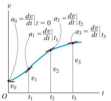
v−t (Velocity vs. Time): The slope of the tangent line represents the instantaneous acceleration, while the area under the curve represents the displacement.
a−t (Acceleration vs. Time): The area under the curve represents the change in velocity (Δv).
A velocity-time graph illustrating the concept of acceleration as the derivative of velocity with respect to time at different points.
Displacement-Based Graphs ($v-s, a-s$)
Sometimes, motion is described in terms of position rather than time.
v−s (Velocity vs. Displacement): These graphs are useful for finding acceleration when a is a function of s.
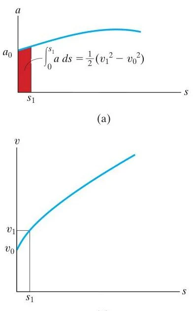
a−s (Acceleration vs. Displacement): These are often used to determine the velocity of a particle at a specific location.
The top graph shows acceleration as a function of displacement, with the integral representing the change in kinetic energy. The bottom graph shows velocity as a function of displacement.
Worked Example: Variable Acceleration
Problem: A car moves such that its velocity is v=(0.6t2+t) m/s. If s=0 when t=0, find the position and acceleration at t=3 s.
Solution:
Find Position (s): Since $v = ds/dt$, we integrate the velocity function with respect to time:
\int_{0}^{s} ds &= \int_{0}^{t} (0.6t^2 + t) dt \\
s &= [0.2t^3 + 0.5t^2]_0^t \\
s &= 0.2t^3 + 0.5t^2
\end{aligned}$$
At $t=3 \text{ s}$:
$$s = 0.2(3)^3 + 0.5(3)^2 = 5.4 + 4.5 = 9.9 \text{ m}$$
2. **Find Acceleration ($a$):** Since $a = dv/dt$, we differentiate the velocity function:
$$\begin{aligned}
a &= \frac{d}{dt}(0.6t^2 + t) \\
a &= 1.2t + 1
\end{aligned}$$
At $t=3 \text{ s}$:
$$a = 1.2(3) + 1 = 4.6 \text{ m/s}^2$$
> **Note:** Because the acceleration is a function of time ($a = 1.2t + 1$), the standard constant acceleration formulas **cannot** be used for this problem.
$$$
$$$
Keep reading for free.
Create an account to finish this reading and make it part of your study routine.