Introduction to Quantitative Analysis for Decision Making
This guide explains quantitative analysis, a scientific approach to managerial decision-making using mathematical and statistical techniques. It covers the process, model development, data integrity, break-even analysis, sensitivity analysis, and common pitfalls.
In the modern business landscape, managers are constantly faced with complex decisions that can determine the success or failure of an organization. While intuition and experience are valuable, they are often insufficient when dealing with large volumes of data or high levels of uncertainty. This is where quantitative analysis becomes essential.
Quantitative analysis is a scientific approach to managerial decision-making in which raw data are manipulated or processed into meaningful, actionable information. Rather than relying on guesswork, this approach uses mathematical and statistical techniques to provide a structured foundation for making choices.
The Quantitative Analysis Approach
The quantitative analysis process is not a single action but a structured sequence of steps designed to move from a vague problem to a concrete, implemented solution. Understanding this flow is critical for any analyst to ensure that the final decision is based on sound logic and accurate data.
The standard sequence includes:
Defining the Problem: Identifying the core issue that requires a solution.
Developing a Model: Creating a mathematical representation of the business situation.
Acquiring Input Data: Gathering the necessary numbers to populate the model.
Developing a Solution: Finding the optimal solution (the best possible outcome) using various mathematical methods.
Testing the Solution: Validating both the data and the model for accuracy and logic.
Analyzing the Results: Studying the implications of the solution and how it might change under different conditions.
Implementing the Results: Putting the analyzed solution into practice.
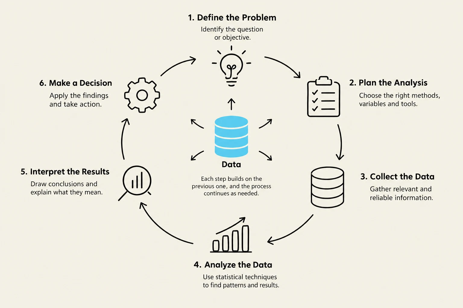
This diagram illustrates a six-step process for data analysis, starting with defining the problem and ending with making a decision based on the interpreted results.
Developing a Mathematical Model
A model is a realistic, solvable, and understandable mathematical representation of a business situation. Models are generally categorized into two types: deterministic models, where all parameters are known with certainty (such as break-even or linear programming models), and probabilistic models, which involve risk and uncertainty (such as decision analysis models).
To build a model, you must understand its three primary components:
Variables: Measurable quantities that can change. A specific type called decision variables are those controlled by the decision-maker (e.g., how many units to produce).
Parameters: Constant, known values used within the model (e.g., the cost of raw materials).
Equations/Inequalities: The mathematical relationships that define the objective or the constraints.
Example: Linear Programming Model
In a linear programming model, a manager might try to maximize profit subject to certain constraints, such as labor hours or machine capacity. For example:
Maximize Profit:
Z=70T+50C
Subject to:
4T+3C2T+1CT,C≤240≤100≥0
In this scenario, T and C are decision variables representing the number of tables and chairs produced, while the numbers (70, 50, 4, 3, etc.) are parameters.
Data Integrity and the GIGO Rule
The quality of your model is entirely dependent on the quality of your input data. Input data can be sourced from company reports, employee interviews, statistical sampling, or direct measurements.
However, analysts must be wary of the GIGO rule: Garbage In, Garbage Out. This principle states that if you use improper, inaccurate, or incomplete data to populate your model, the resulting "optimal solution" will be misleading and potentially harmful to the organization.
Exam Tip: When testing a solution, always check two things: the accuracy of the input data (is the number correct?) and the logic of the model (does the math actually represent the real-world situation?).
Practical Application: Break-Even Analysis
One of the simplest and most common models is the break-even model. This is a deterministic model used to find the point where total revenue equals total costs, resulting in zero profit.
Worked Example
A company sells rebuilt springs for $8 per unit (s). The fixed cost (f) to equip the factory is $$1,000$, and the variable cost (v) per unit is $3.
Develop the Profit Model:
Profit is Revenue minus Expenses (Fixed Costs + Variable Costs).
Find the Break-Even Point (BEP):
To break even, set Profit to 0:
01000X=5X−1000=5X=200 units
The company must sell 200 units to avoid a loss.
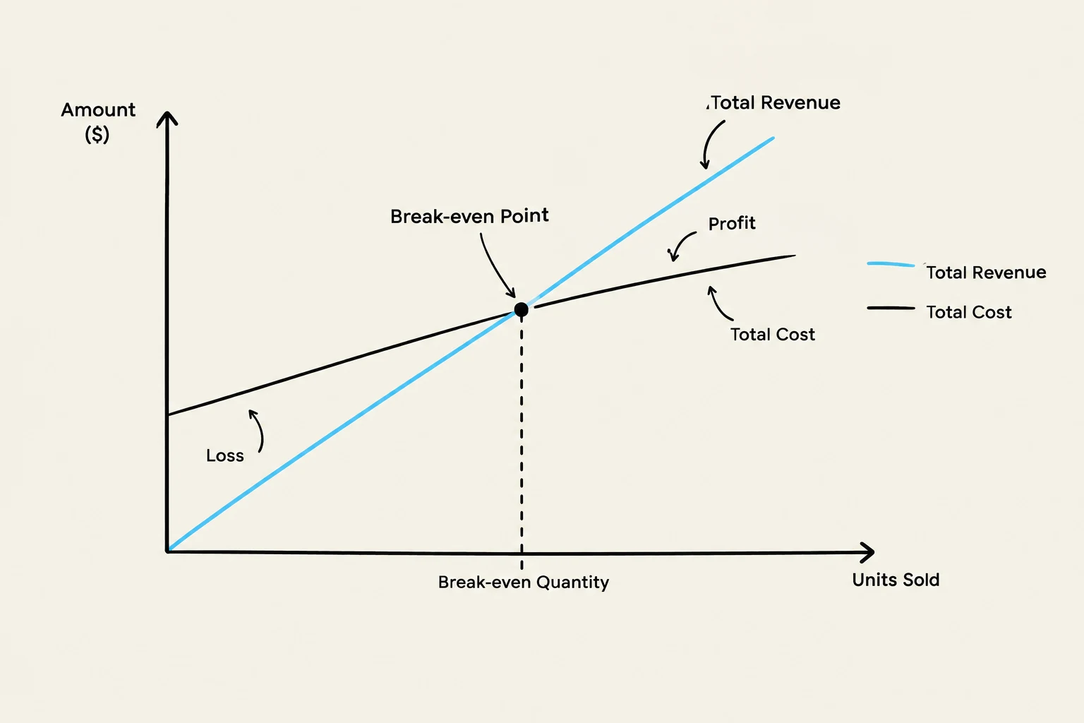
This graph illustrates the break-even point in economics, showing the intersection of total revenue and total cost curves. To the left of the break-even point, the business incurs a loss, while to the right, it generates a profit.
Analyzing Results and Sensitivity Analysis
Once a solution is found, the analyst must determine its implications. This is where sensitivity analysis (also known as post-optimality analysis) comes into play.
Sensitivity analysis studies how much the optimal solution changes if the input data or model parameters are altered.
A sensitive model is one where a very small change in an input (like a slight increase in material costs) leads to a significant change in the optimal decision.
If a model is highly sensitive, the analyst must be extremely careful to ensure that the input data is as accurate as possible.
Tools for Quantitative Analysis
Modern analysts rarely perform these complex calculations by hand. Software tools like Microsoft Excel are industry standards.
Data Analysis ToolPak: Useful for regression models.
Solver: An algorithm-based tool used to find optimal solutions for linear programming and other complex problems.
Excel QM: A specialized add-in designed specifically for quantitative analysis management.
Summary of Potential Pitfalls
While powerful, quantitative analysis has limitations that managers must recognize:
Complexity vs. Understanding: A model that is too complex may be difficult for stakeholders to trust or understand.
Simplification Errors: To make models solvable, we often assume certain things are constant (like assuming everything produced is immediately sold), which may lack real-world accuracy.
Single-Answer Limitation: Most models provide one "optimal" answer, whereas managers often prefer a range of viable options.
Keep reading for free.
Create an account to finish this reading and make it part of your study routine.