In statistics, we often work with data collected from a sample, but our ultimate goal is to understand the larger population from which that sample was drawn. Probability serves as the essential mathematical bridge between these two worlds. By understanding the likelihood of various outcomes, we can make informed inferences about the population based on the limited information available in our data.
The Building Blocks: Experiments, Spaces, and Events
To study probability, we must first define the environment in which we are working. This begins with a random experiment, which is a process where the specific result is unknown in advance, even though we know the set of all possible results.
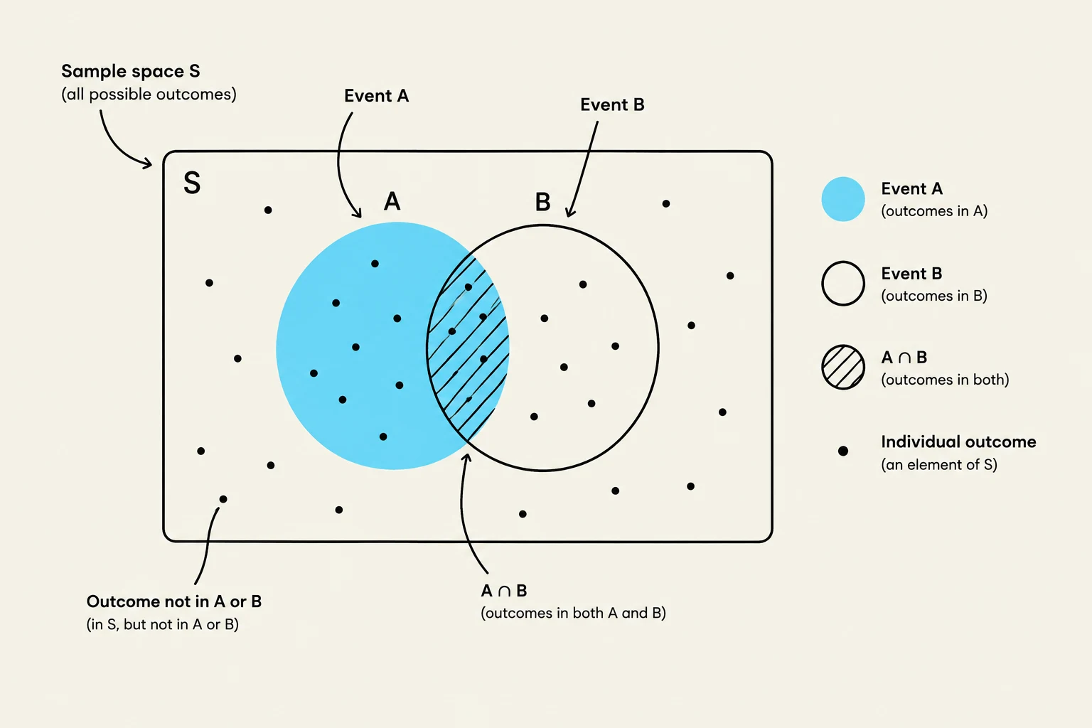
The collection of every possible result from an experiment is called the sample space (S). Each individual result that can occur is known as an outcome. Within this sample space, we are often interested in specific collections of outcomes, which we call events. An event is simply any subset of the sample space; we say the event "occurs" if the actual outcome of the experiment is a member of that subset.
This Venn diagram illustrates the concepts of sample space, events, and outcomes in probability theory. It shows two events, A and B, within a sample space S, and their intersection, representing outcomes common to both events.
Operations on Events
We can manipulate events using three fundamental operations:
Union (A∪B): Represents "A or B." This event occurs if at least one of the events occurs (it could be A, it could be B, or it could be both).
Intersection (A∩B): Represents "A and B." This event occurs only if both events occur simultaneously.
Complement (Ac): Represents "not A." This event occurs if A does not occur.
The Rules of Probability
Probability is the assignment of a number P(A) to an event A. For these assignments to be mathematically sound, they must obey three fundamental axioms:
Non-negativity and Boundedness: For any event A, 0≤P(A)≤1.
Certainty: The probability of the entire sample space is P(S)=1.
Additivity for Mutually Exclusive Events: If two events A and B are mutually exclusive (meaning they cannot both occur, so A∩B=∅), then the probability of either occurring is the sum of their individual probabilities: P(A∪B)=P(A)+P(B).
Exam Tip: Always check if events are mutually exclusive before adding their probabilities. If they can overlap, you must use the General Addition Rule to avoid double-counting the intersection.
The General Addition Rule and Complement Rule
When events are not mutually exclusive, we use the general addition rule to account for the overlap:
P(A∪B)=P(A)+P(B)−P(A∩B)
By subtracting the intersection, we ensure that the outcomes belonging to both A and B are only counted once. Additionally, the complement rule allows us to find the probability of an event not occurring quite easily: P(Ac)=1−P(A).
Conditional Probability and Independence
Often, we want to know the probability of an event given that we already have some information. This is known as conditional probability. For any event B where P(B)>0, the probability of A given B is:
P(A∣B)=P(B)P(A∩B)
From this definition, we can derive the multiplicative rule, which is useful for calculating the probability of two events happening together:
P(A∩B)=P(A∣B)P(B)=P(B∣A)P(A)
Independence
Two events are considered independent if the occurrence of one does not change the probability of the other. Mathematically, A and B are independent if:
P(A∣B)=P(A)⟺P(A∩B)=P(A)P(B)
Note that "mutually exclusive" and "independent" are very different concepts: if two events are mutually exclusive, they are actually highly dependent, because if one happens, the probability of the other happening becomes zero.
Advanced Probability: Partitions and Bayes' Rule
A partition of a sample space is a set of events that are both mutually exclusive and exhaustive, meaning they do not overlap and they cover the entire sample space S. The simplest partition is ${A, A^c}$.
The Law of Total Probability (LTP)
If we have a partition, we can find the total probability of an event B by summing its conditional probabilities across all parts of the partition:
P(B)=P(B∣A)P(A)+P(B∣Ac)P(Ac)
This is often visualized using a probability tree, where you multiply probabilities along the branches and add the results of the different paths.
This is a probability tree diagram illustrating conditional probabilities and event complements in a sample space.
Bayes' Rule
Bayes' Rule is a powerful tool that allows us to "reverse" conditional probabilities. If we know P(B∣A) but want to find P(A∣B), we use:
P(A∣B)=P(B)P(B∣A)P(A)
When P(B) is not directly provided, we substitute the Law of Total Probability into the denominator.
Caution: The Base-Rate Fallacy. A common mistake is to judge P(A∣B) based solely on the accuracy of the condition P(B∣A), while ignoring the "base rate" or the initial probability P(A). For example, even a highly accurate medical test may yield a low probability of actual disease if the disease itself is extremely rare.
Keep reading for free.
Create an account to finish this reading and make it part of your study routine.