This material introduces the mathematics of probability, describing experiments through sample spaces and events while quantifying uncertainty associated with outcomes. It covers basic rules and concepts like randomness, probability quantification, and prediction versus result.
In our daily lives, we are constantly surrounded by uncertainty. Whether we are predicting the weather, the outcome of a sports match, or the results of a scientific experiment, we often encounter situations where the exact outcome is unknown. This unpredictability is what we call randomness.
While randomness can feel chaotic, it is not necessarily lawless. In many cases, apparent randomness arises from our limited knowledge of a complex system or from inherent "pure" randomness found in the fundamental laws of nature, such as quantum mechanics. To make sense of this uncertainty, we use statistical methods underpinned by the mathematics of probability.
Understanding Randomness
Randomness embodies the ideas of both unpredictability and disorder. If an event has no discernible pattern and its outcome cannot be predicted, it is considered random.
In practical applications, such as biology or engineering, we treat any system whose outcome we cannot predict as random. By applying the tools of probability, we can move from mere guesswork to a structured way of interpreting and predicting experimental observations.
Describing Experiments: Sample Spaces and Events
To perform probabilistic calculations, we must first define the framework of the experiment. This is done using two fundamental concepts: the sample space and events.
The Sample Space (S)
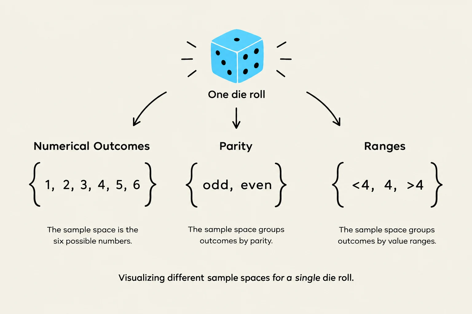
This diagram illustrates the concept of sample spaces for a single die roll, categorizing outcomes by numerical values, parity (odd/even), and value ranges.
The sample space, denoted by S, is the collection of all possible outcomes of an experiment. It is important to note that the definition of a sample space depends entirely on what you are measuring.
For example, if you roll a single six-sided die, your sample space could be:
The specific numbers: $S = {1, 2, 3, 4, 5, 6}$
The parity: S={odd, even}
Ranges: $S = {<4, 4, >4}$.
Events
Venn diagram showing overlapping and disjoint events.
An event is a subset of the sample space representing specific outcomes of interest. For instance, in a die roll where $S = {1, 2, 3, 4, 5, 6}$, the event "rolling a 1 or 2" would be the subset ${1, 2}$.
Events can be categorized by how they relate to one another:
Disjoint (Mutually Exclusive) Events: These are events that cannot occur at the same time. For example, rolling a number <3 and a number ≥3 are disjoint events.
Overlapping Events: These are events that share common outcomes. For example, in a die roll, the event "rolling an even number" ${2, 4, 6}$ and the event "rolling a number >3" ${4, 5, 6}$ overlap because they both contain the outcomes 4 and 6.
Logical Operations and Set Theory
We can combine events using logical operations, which are often expressed using set theory notation:
'And' (Intersection ∩): The event that both A and B occur.
'Or' (Union ∪): The event that either A occurs, B occurs, or both occur.
'Not' (Complement $A'$): The event that A does not occur.
Set theory notationFigure 1: Set theory notation.
Quantifying Probability
Probability is the quantitative measure of the uncertainty associated with events. It can be expressed in several ways, including percentages, fractions, decimals between 0 and 1, or as an odds ratio (e.g., a $75%$ probability can be written as 0.75, 3/4, or odds of $3:1$).
Conceptually, probability can represent:
The chance of an outcome in a single trial.
The frequency of an outcome in repeated trials.
A degree of belief in an outcome.
Probability in Discrete Systems
In a discrete system where all outcomes in the sample space are equally likely, the probability of an event A occurring, denoted as P(A), is the ratio of the size of the event to the size of the sample space:
P(A)=size of Ssize of A
Or, more intuitively:
P(A)=Total number of possible outcomesNumber of outcomes in A
Key Boundaries
Impossible events: An event that cannot happen has a probability of 0.
Certain events: An event that is guaranteed to happen has a probability of 1.
Prediction vs. Result
This illustration demonstrates the concept of random deviation in probability. The left side shows a predicted outcome of 5 heads and 5 tails in 10 coin flips, representing an expected average. The right side shows the actual outcome of 4 heads and 6 tails, illustrating how random chance can lead to results that differ from the prediction.
A common pitfall in understanding probability is confusing a prediction with a result. Probability allows us to predict the most likely outcomes over many trials, but individual results are subject to randomness.
Example: If you toss a fair coin ten times, the most likely prediction is 5 heads and 5 tails. However, if you actually perform the experiment and get 4 heads and 6 tails, this does not mean your probability calculation was wrong; it simply means the individual result deviated from the expected average due to inherent randomness.
Summary of Basic Rules
To solve more complex problems, keep these fundamental properties in mind:
The Range Rule: For any event A, 0≤P(A)≤1.
The Addition Rule (for 'Or'):P(A∪B)=P(A)+P(B)−P(A∩B)
We subtract the intersection P(A∩B) to avoid counting the overlapping outcomes twice.
Disjoint Addition: If A and B are disjoint, then P(A∩B)=0, so:
P(A∪B)=P(A)+P(B)
The Complement Rule (for 'Not'):P(A′)=1−P(A)
Keep reading for free.
Create an account to finish this reading and make it part of your study routine.