An introduction to econometrics, covering the empirical analysis process, distinguishing correlation from causation, types of data (cross-sectional, time-series, panel), and methods for visualizing and describing data.
Econometrics is a vital tool in the economist's toolkit, providing the statistical methods necessary to estimate economic relationships, test theoretical models, and evaluate the effectiveness of business or government policies. While statistics provides the mathematical foundation, econometrics applies these tools specifically to the complexities of economic data to turn abstract theories into measurable realities.
The Process of Empirical Analysis
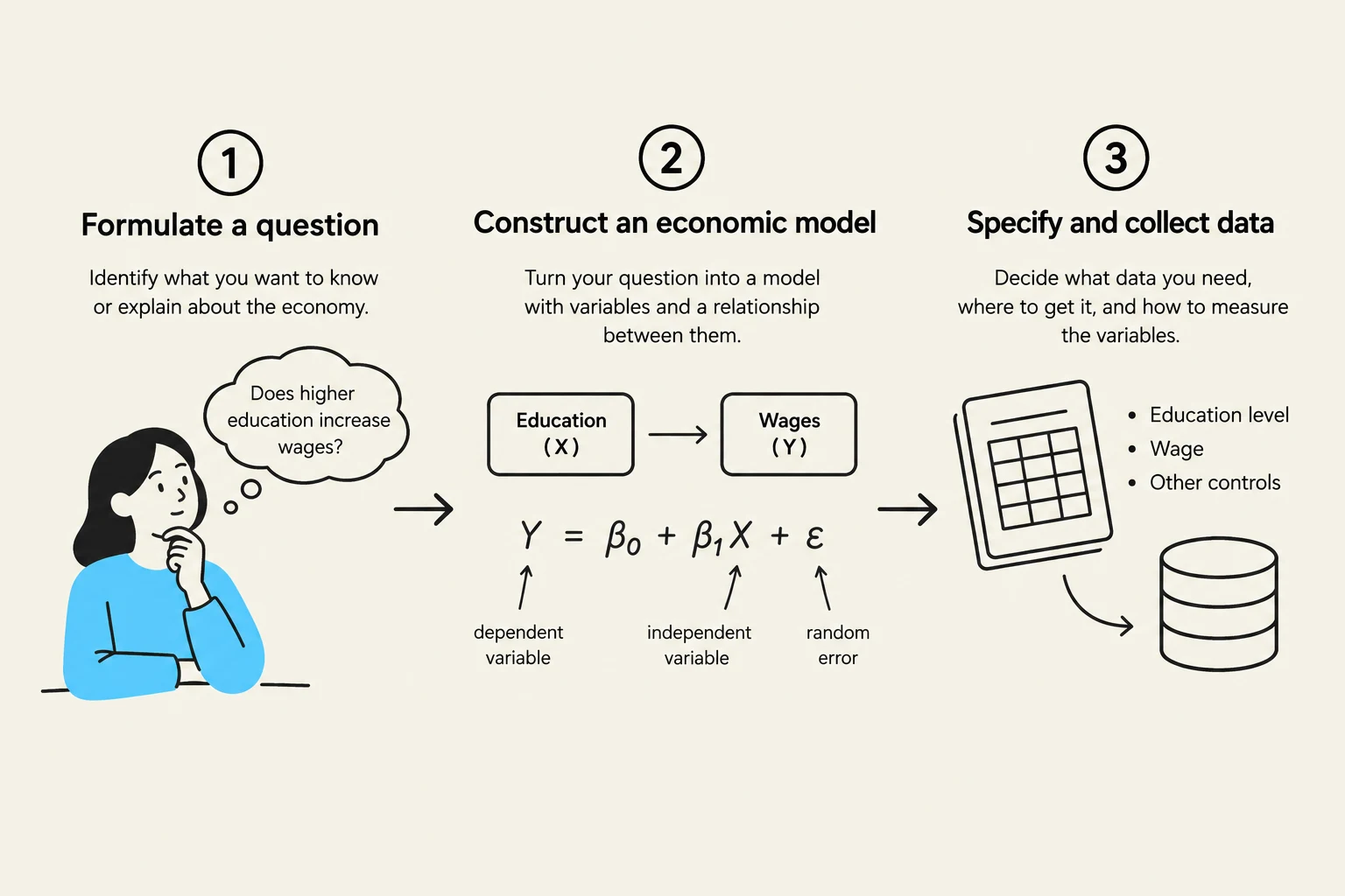
To move from a theoretical idea to a concrete conclusion, researchers follow a structured process known as empirical analysis. This process typically involves three primary steps:
Formulating a question: Identifying a specific economic problem, such as "Does increasing education lead to higher wages?".
Developing an economic model: Creating an informal framework of how variables interact. For example, we might assume that $wage = f(educ, exper, training)$.
Specifying an econometric model: Converting the informal model into a mathematical equation that can be tested with data.
An econometric model takes the form of a regression equation:
wage=β0+β1educ+β2exper+β3training+u
In this equation, β0,β1,… are the parameters we wish to estimate. These parameters represent the strength and direction of the relationship between the independent variables (like education) and the dependent variable (wage). The term u is the error term, which accounts for all other unobserved factors that might influence wages but are not explicitly included in the model.
To find these parameters, researchers gather a random sample—a smaller, representative version of the larger population. They then apply regression methods, most commonly Ordinary Least Squares (OLS), to calculate estimates for the parameters. Once these estimates are obtained, researchers perform inference to determine if the results are statistically significant for the broader population and check if the results are robust.
This diagram illustrates the three key steps in constructing an economic model: formulating a question, constructing the model with variables and their relationships, and specifying and collecting relevant data.
Causal Effects vs. Correlation
One of the most important distinctions in econometrics is the difference between correlation and causation. A causal effect occurs when a specific action or treatment directly results in a measurable change in an outcome.
The gold standard for measuring causality is the randomized controlled experiment. In such an experiment, subjects are randomly assigned to either a treatment group (which receives the action) or a control group (which does not). This randomness ensures that, on average, the two groups are identical in every way except for the treatment. The causal effect is then calculated as:
Exam Tip: Remember that correlation is merely a description of how two variables move together in a dataset. It does not prove that one variable causes the other.
In the real world, we often rely on observational data—data collected by observing behavior as it naturally occurs without intervention. Because we cannot always run experiments, we run into the risk of mistaking correlation for causation due to three main issues:
Omitted (confounding) factors: An unobserved variable influences both the supposed cause and the effect.
Reverse causality: The direction of influence is the opposite of what was assumed; the "effect" is actually causing the "cause".
Selection: The groups being compared are not similar because of how individuals "selected" themselves into a group (non-random assignment).
It is also important to distinguish causation from prediction. Prediction (or forecasting) involves using known variables to estimate the value of an unknown variable, such as predicting next year's GDP growth. While a good prediction model is highly useful, it does not necessarily explain the underlying causal mechanism.
Data Sources and Structures
Data in econometrics generally comes from two sources: experimental data, derived from designed trials to investigate causality, and observational data, obtained from real-world observations.
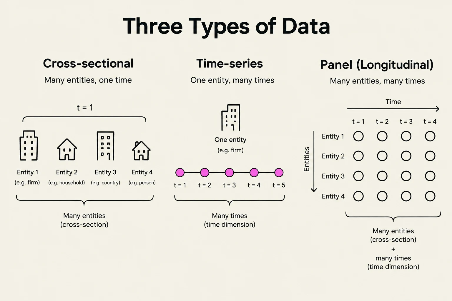
Regardless of the source, data is organized in a rectangular format where each row represents an observation and each column represents a variable. Economists categorize these datasets into three primary types:
Cross-sectional data: Observations of multiple entities (such as individuals, firms, or countries) at a single point in time.
Time-series data: Observations of a single entity (such as one country's GDP) over multiple consecutive time periods.
Panel data (also called longitudinal data): A combination of both, where multiple entities are observed over multiple time periods.
This diagram illustrates three types of data: cross-sectional (many entities, one time), time-series (one entity, many times), and panel/longitudinal (many entities, many times).
Visualizing and Describing Data
Before running complex regressions, economists must understand the "shape" and "center" of their data. For quantitative data, we often use a histogram to see the distribution of values. Common shapes include symmetric distributions and right-skewed distributions (where a long tail stretches to the right, common in wealth and income data).
To summarize a dataset, we look at measures of central tendency and variability:
Central Tendency: The mean (arithmetic average), the median (the middle value), and the mode (the most frequent value). Note that the median is often more robust (resistant to outliers) than the mean.
Variability: The range (difference between max and min), variance (sX2), and standard deviation (sX) describe how spread out the data is.
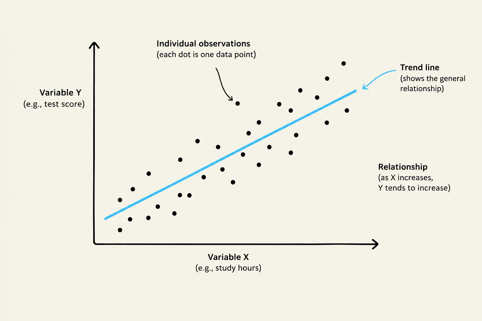
Finally, to understand the relationship between two variables, we use a scatterplot. From this, we can calculate the sample correlation coefficient (rXY), which measures the strength and direction of a linear relationship on a scale from −1 to +1.
A scatter plot illustrating the relationship between two variables, Variable X (e.g., study hours) and Variable Y (e.g., test score), with a trend line showing a general positive correlation.
Keep reading for free.
Create an account to finish this reading and make it part of your study routine.