This article introduces consumer theory in microeconomics, explaining how individuals make choices based on preferences and budget constraints. It details preference relations (strict, indifference, weak), the axioms of consistency (completeness, reflexivity, transitivity), and visualizes preferences using indifference
In microeconomics, we often want to understand why people buy what they buy. To do this, we use Consumer Theory, a mathematical framework designed to model how individuals make choices. The theory operates on a simple behavioral postulate: a decision-maker will always choose the most preferred alternative from the set of all available options.
To model this behavior, economists separate the problem into two distinct parts. First, we must understand what a consumer wants to do, which is defined by their Preferences. Second, we must understand what they can do, which is defined by their Budget Constraint. This article focuses on the first part: how we mathematically represent the desirability of different consumption bundles.
Preference Relations and Ordinality
When we talk about preferences, we aren't necessarily measuring "utility" in terms of happiness units (like "I am 10 units happy"). Instead, we use ordinal relations. This means we are simply ranking consumption bundles—such as X=(x1,x2) and Y=(y1,y2)—in order of their desirability.
There are three primary ways a consumer can relate two bundles:
Strict Preference (X≻Y): The consumer prefers bundle X over bundle Y. They would rather have X than Y.
Indifference (X∼Y): The consumer finds both bundles equally satisfactory. They are just as happy with X as they are with Y.
Weak Preference (X⪰Y): The consumer considers X to be at least as good as Y. This is a broader category that includes both strict preference and indifference.
These relations are mathematically interconnected. For example, if a consumer thinks X is at least as good as Y (X⪰Y) and also thinks Y is at least as good as X (Y⪰X), they must be indifferent between the two (X∼Y).
Exam Tip: Remember that "weak preference" is the "umbrella" term. If X≻Y, then it is also true that X⪰Y. However, if X⪰Y, it does not necessarily mean X≻Y (because they might be indifferent).
The Axioms of Consistency
For consumer theory to be useful for prediction, we cannot have consumers who change their minds randomly or behave illogically. We assume that preferences follow certain axioms to ensure consistency.
Completeness
The Completeness Axiom states that for any two bundles X and Y, a consumer must be able to compare them. They must be able to say X⪰Y, Y⪰X, or X∼Y. There is no "I don't know" in standard consumer theory; the consumer always has a ranking.
Reflexivity
The Reflexivity Axiom is a fundamental logical requirement: any bundle is at least as preferred as itself (X⪰X).
Transitivity
The Transitivity Axiom ensures logical consistency in rankings. If a consumer prefers X to Y and prefers Y to Z, they must also prefer X to Z. Without transitivity, a consumer could get stuck in a "preference loop," making it impossible to determine a "best" choice.
This diagram illustrates the concept of transitivity in preferences, showing that if X is preferred to Y and Y is preferred to Z, then X is necessarily preferred to Z.
Visualizing Preferences: Indifference Curves
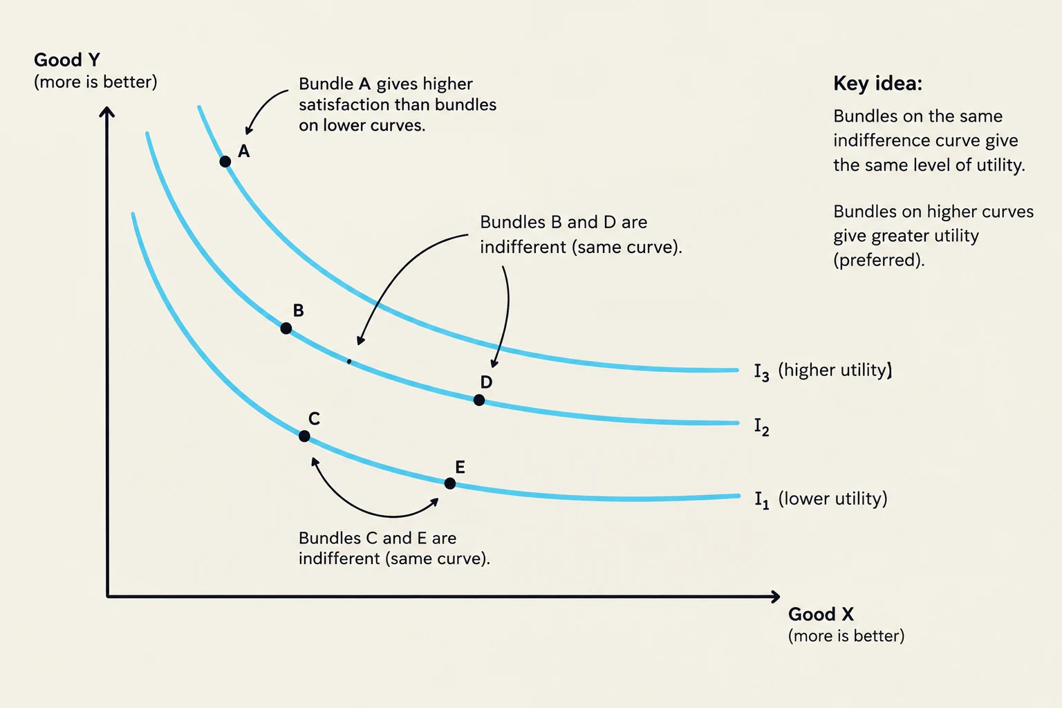
To visualize these rankings, economists use Indifference Curves (or indifference sets). An indifference curve represents a set of all consumption bundles that provide the same level of satisfaction to the consumer.
If you are on the same indifference curve, you are indifferent between all points on that curve. Bundles located on "higher" indifference curves (further from the origin, assuming goods) are strictly preferred to bundles on "lower" curves.
This graph illustrates indifference curves in economics, showing how combinations of two goods (Good X and Good Y) can provide different levels of utility or satisfaction. Bundles on the same curve offer equal utility, while bundles on higher curves are preferred.
The Shape of Preferences
The slope of an indifference curve tells us about the relationship between the two goods:
Goods: If both items are "goods" (more is better), the curves are downward sloping.
Bads: If one item is a "bad" (less is better), the curve may slope upward.
Perfect Substitutes: If a consumer views two goods as interchangeable, the indifference curves are straight lines with a constant slope.
Perfect Complements: If goods must be consumed in fixed proportions (like left shoes and right shoes), the curves are L-shaped.
The Marginal Rate of Substitution (MRS)
A crucial concept derived from indifference curves is the Marginal Rate of Substitution (MRS). The MRS measures the rate at which a consumer is willing to substitute one good for another while maintaining the same level of satisfaction.
Mathematically, the MRS is the absolute value of the slope of the indifference curve at a specific point:
MRS=−dx1dx2
In practical terms, if the MRS is 2, the consumer is willing to give up 2 units of good x2 to get 1 additional unit of good x1 without feeling better or worse off.
Key Concept: Convexity and Diminishing MRS
Most "well-behaved" preferences are convex. This means that as you consume more of x1, you are willing to give up less and less of x2 to get even more x1. This is known as a diminishing marginal rate of substitution.
This graph illustrates an indifference curve, showing the trade-off between two goods (Good X and Good Y) for a consumer. The slope of the curve, representing the Marginal Rate of Substitution (MRS), decreases as the consumer consumes more of Good X and less of Good Y.
By combining these preference relations, axioms, and geometric tools, economists can build complex models to predict how changes in prices or income will shift a consumer's optimal choice.
Keep reading for free.
Create an account to finish this reading and make it part of your study routine.