This content introduces the fundamental concepts of combinatorics and probability, explaining how to count outcomes using permutations and combinations to calculate the likelihood of events. It covers sample spaces, discrete vs. continuous events, and provides worked examples.
In our daily lives, we often encounter uncertainty—whether we are predicting the weather, the outcome of a sports match, or the results of a scientific experiment. To make sense of this randomness, mathematicians use the tools of probability. At the heart of probability lies combinatorics, the branch of mathematics dedicated to counting the number of ways specific events can occur. By mastering the art of counting, we can define the size of possible outcomes and ultimately calculate the likelihood of specific events.
The Foundation: Sample Spaces and Events
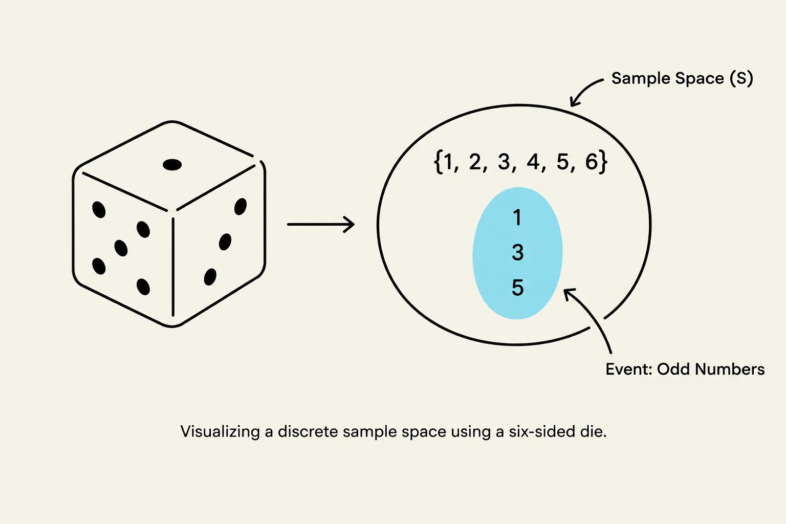
Visualizing a discrete sample space using a six-sided die, showing the sample space S and the event of odd numbers.
Before we can count, we must define what we are counting. In probability, we describe the various possible outcomes of an experiment as events, and the collection of all possible outcomes is known as the sample space (S).
The sample space can be defined in different ways depending on the experiment. For example, if you roll a single six-sided die, your sample space could be the set of numbers ${1, 2, 3, 4, 5, 6}$, or it could be categorized as {odd, even}.
Probability is essentially a way of quantifying the "size" of an event relative to the size of the sample space:
P(A)=size of sample space Ssize of event A
Discrete vs. Continuous Sample Spaces
How we calculate these "sizes" depends on the nature of the data:
Discrete events: These involve countable outcomes, such as the number of heads in ten coin tosses or the result of a die roll. In a discrete system, a probability of 0 means an event is impossible, and a probability of 1 means it is certain.
Continuous sample spaces: These involve outcomes that can take any value within a range, such as measuring the exact time between bus arrivals. In continuous systems, the probability of any single, exact outcome (e.g., a bus arriving at exactly 12.0000... minutes) is 0; instead, we calculate probabilities over a specific range.
Exam Tip: Galton's Paradox
When working with discrete sample spaces, always ensure that all fundamental units (outcomes) are counted equally. If you fail to count outcomes evenly, you may fall into "Galton's paradox," where intuitive but incorrect conclusions are drawn because the underlying sample space was not properly partitioned.
Combinatorics: The Mathematics of Counting
This illustration compares permutations, where order matters, with combinations, where order does not matter, using colored circles as examples.
The primary distinction in combinatorics is whether the order of elements matters. This leads us to two fundamental concepts: permutations and combinations.
Permutations: When Order Matters
A permutation is a particular ordering of elements. If you are arranging books on a shelf or assigning specific roles to people, the order is vital.
1. Arranging n Distinct Items
To find the number of ways to arrange n unique items, we use n factorial, denoted as $n!$. The factorial is the product of all positive integers up to n:
n!=n×(n−1)×⋯×1
By mathematical definition, $0! = 1$.
2. Selecting k items from n Distinct Items
If you have a larger set of n items but only want to select and order a subset of k elements, the formula is:
nPk=(n−k)!n!
3. Permutations with Distinct Subgroups
Sometimes, a set contains items that are not all unique. If a set of n items contains j distinct subgroups of sizes k1,k2,…,kj where elements within a subgroup are indistinguishable (such as arranging the letters in a word where some letters repeat), the number of unique permutations is:
Pk1,k2,…,kjn=k1!k2!…kj!n!
Combinations: When Order Does Not Matter
In many scenarios, the order of selection is irrelevant. For instance, if you are choosing three flavors of ice cream for a bowl or selecting a committee of four people from a group, the group is the same regardless of who was picked first.
Because different orderings of the same elements are considered identical in combinations, we "divide out" the extra permutations. The formula for choosing k elements from n is:
nCk=(kn)=k!(n−k)!n!
A useful property to remember for calculations is symmetry: (kn)=(n−kn). This means choosing 2 people to go on a trip is mathematically the same as choosing n−2 people to stay home.
Applying Counting to Probability
Once we have used combinatorics to find the number of successful outcomes and the total number of outcomes in the sample space, calculating probability becomes straightforward.
For independent events, such as flipping a coin multiple times, the total number of permutations is 2n, where n is the number of tosses.
Worked Example: The Die Roll
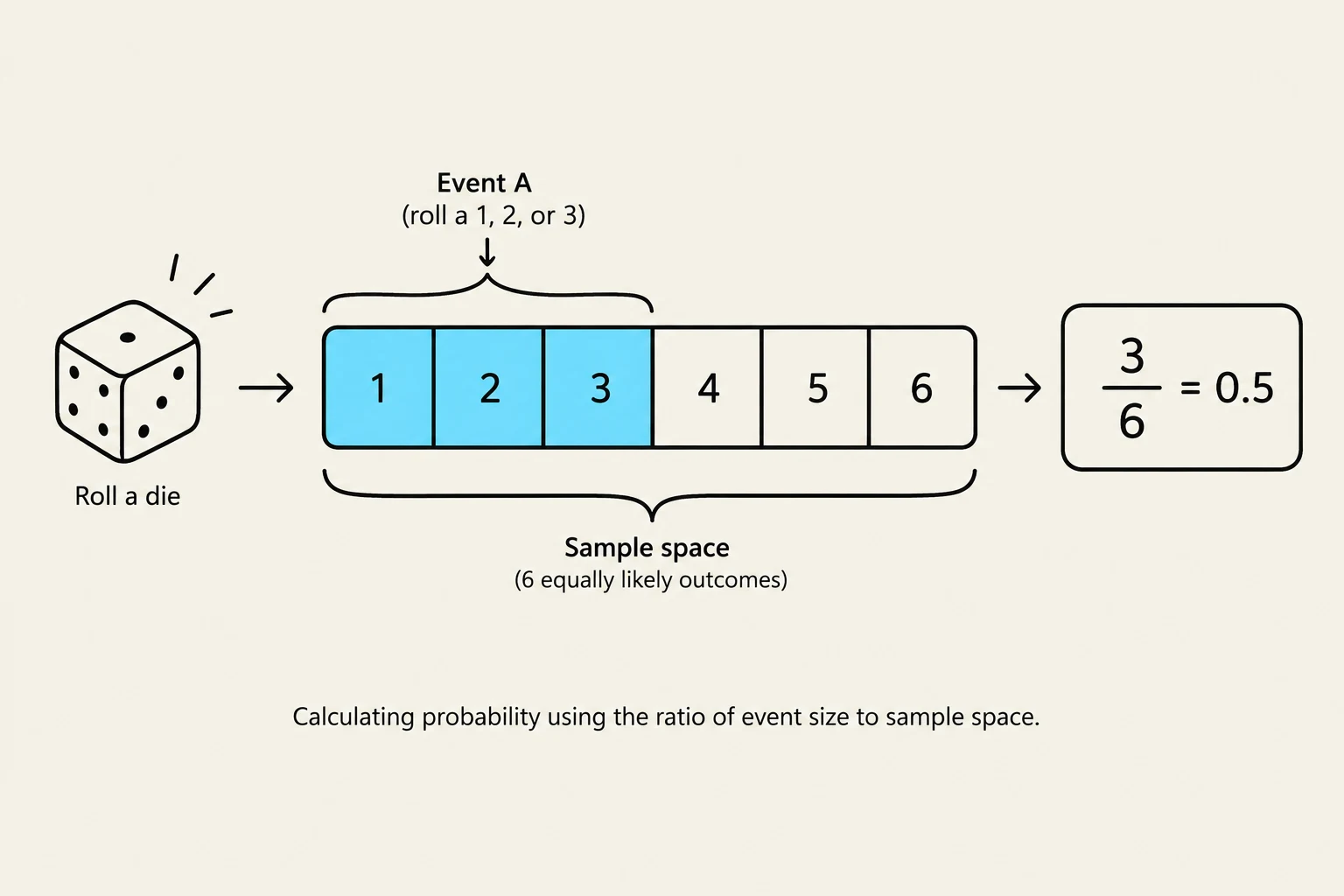
This diagram illustrates how to calculate the probability of an event using a standard six-sided die. It shows that the probability of rolling a 1, 2, or 3 (Event A) is 3 out of 6 possible outcomes, which simplifies to 0.5.
Suppose you want to find the probability of rolling a number less than 4 on a single fair die.
Identify the Sample Space (S): ${1, 2, 3, 4, 5, 6}$. Total outcomes = 6.
By combining the logic of counting (combinatorics) with the framework of the sample space, we can navigate through complex, random systems with mathematical precision.
Keep reading for free.
Create an account to finish this reading and make it part of your study routine.