Introduction to Biostatistics: Confidence Intervals and Statistical Inference
Learn about statistical inference, point estimates, and confidence intervals in biostatistics. Understand the components of confidence interval calculations, including z-scores, standard error of the mean, and variance. Explore factors influencing interval precision like sample size and confidence level, with a worked
In the world of research and evidence-based practice, we rarely have the luxury of measuring every single person in a population. Instead, we take samples and use those samples to make educated guesses about the whole group. This process of using sample data to make generalizations about a larger group is known as statistical inference. However, because we are only looking at a subset of people, our "guess" is never perfect. To account for this uncertainty, biostatisticians use confidence intervals.
The Core Concepts: Point Estimates and Population Parameters
To understand a confidence interval, we must first distinguish between what we know from our sample and what we are trying to discover about the world.
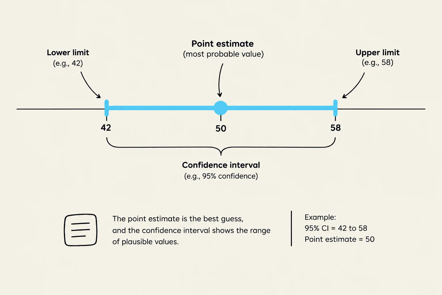
The value we are ultimately interested in is the population parameter—the true, actual value (such as a mean) of the entire group we are studying. Since we cannot measure everyone, we calculate a point estimate from our sample. The point estimate is a single value that serves as our "best guess" or the most probable value for the population.
A confidence interval is a range of values around that point estimate that we are confident contains the true population parameter.
Exam Tip: In a correctly calculated confidence interval, the point estimate must always be located exactly in the middle of the range. If the point estimate is not in the center, there is a mathematical error.
This illustration explains the concepts of point estimate and confidence interval, which are fundamental in statistics for estimating population parameters from sample data. The point estimate represents the single best guess for a parameter, while the confidence interval provides a range of plausible values for that parameter, along with a level of confidence (e.g., 95%).
The Probability Distribution and Sampling
How do we know how "confident" we are? This relies on the concept of a probability distribution, specifically the sampling distribution of means.
If we were to repeat our study an infinite number of times, taking a new sample each time and calculating a new interval, a 95% confidence level means that 95% of those calculated intervals would successfully overlap the true population mean.
It is important to note that not every value within a confidence interval is equally likely to be the true population mean. Because the sampling distribution follows a bell-shaped curve, the values closest to our point estimate are the most probable, and the probability decreases as you move toward the edges of the interval.
The Anatomy of the Equation
While you may not be required to perform complex manual calculations, understanding the components of the confidence interval formula is essential for interpreting research results. The formula is structured as follows:
Confidence Interval=Point Estimate±(z-score⋅SEM)
To understand this, we need to break down three key components:
The z-score: This is a standard deviation unit that represents how many standard errors we are moving away from the mean to achieve a specific level of confidence. For a 95% confidence interval, the z-score is 1.96; for a 90% interval, it is 1.65.
The Standard Error of the Mean (SEM): This measures how much the sample mean is expected to vary from the true population mean. It is calculated using the sample standard deviation and the sample size (n):
SEM=nsample standard deviation
Variance: This refers to the spread or variability of the data.
A normal distribution curve illustrating a point estimate and its corresponding confidence interval on the parameter value axis.
Precision and the Factors that Shape the Interval
In biostatistics, precision refers to how narrow or "tight" the confidence interval is. A narrow interval (e.g., 39 to 41) is considered more precise than a wide interval (e.g., 30 to 50).
Three main factors influence the width (precision) of your interval:
Sample Size (n): As the sample size increases, the precision increases (the interval narrows). Mathematically, because n is in the denominator of the SEM formula, a larger n results in a smaller SEM.
Variance (Standard Deviation): If the data in your sample is very consistent (low variance), your estimate will be more precise. High variability in the data leads to a wider, less precise interval.
Confidence Level: This is often counterintuitive. If you decrease your level of confidence (for example, from 95% down to 90%), your interval becomes narrower and more "precise". However, you are also increasing the risk that your interval fails to actually contain the true population parameter.
Worked Example: Ankle Dorsiflexion
To see these moving parts in action, let's look at a practical example involving ankle dorsiflexion range of motion:
Given Data:
Sample Mean (Point Estimate): 15.6
Sample Standard Deviation: 9
Sample Size (n): 40
Confidence Level: $95%$ (which gives us a z-score of 1.96)
Step 1: Calculate the Standard Error of the Mean (SEM)SEM=409≈1.4
Step 2: Calculate the Margin of ErrorMargin of Error=1.96⋅1.4≈2.7
Step 3: Determine the Confidence IntervalLower Bound=15.6−2.7=12.9Upper Bound=15.6+2.7=18.3
Result: We are 95% confident that the true population mean for ankle dorsiflexion is between 12.9 and 18.3.
Keep reading for free.
Create an account to finish this reading and make it part of your study routine.