Graphing a polynomial function might initially seem like a daunting task, especially when dealing with high-degree equations. However, by breaking the function down into specific components—such as its intercepts, its behavior at those intercepts, and its overall direction—you can sketch an accurate representation of the function without needing to plot dozens of individual points. This article will guide you through the systematic process of polynomial sketching.
Understanding Intercepts
The first step in analyzing any polynomial is to identify where the graph crosses or touches the axes. These points are known as intercepts.
Vertical Intercepts (y-intercept)
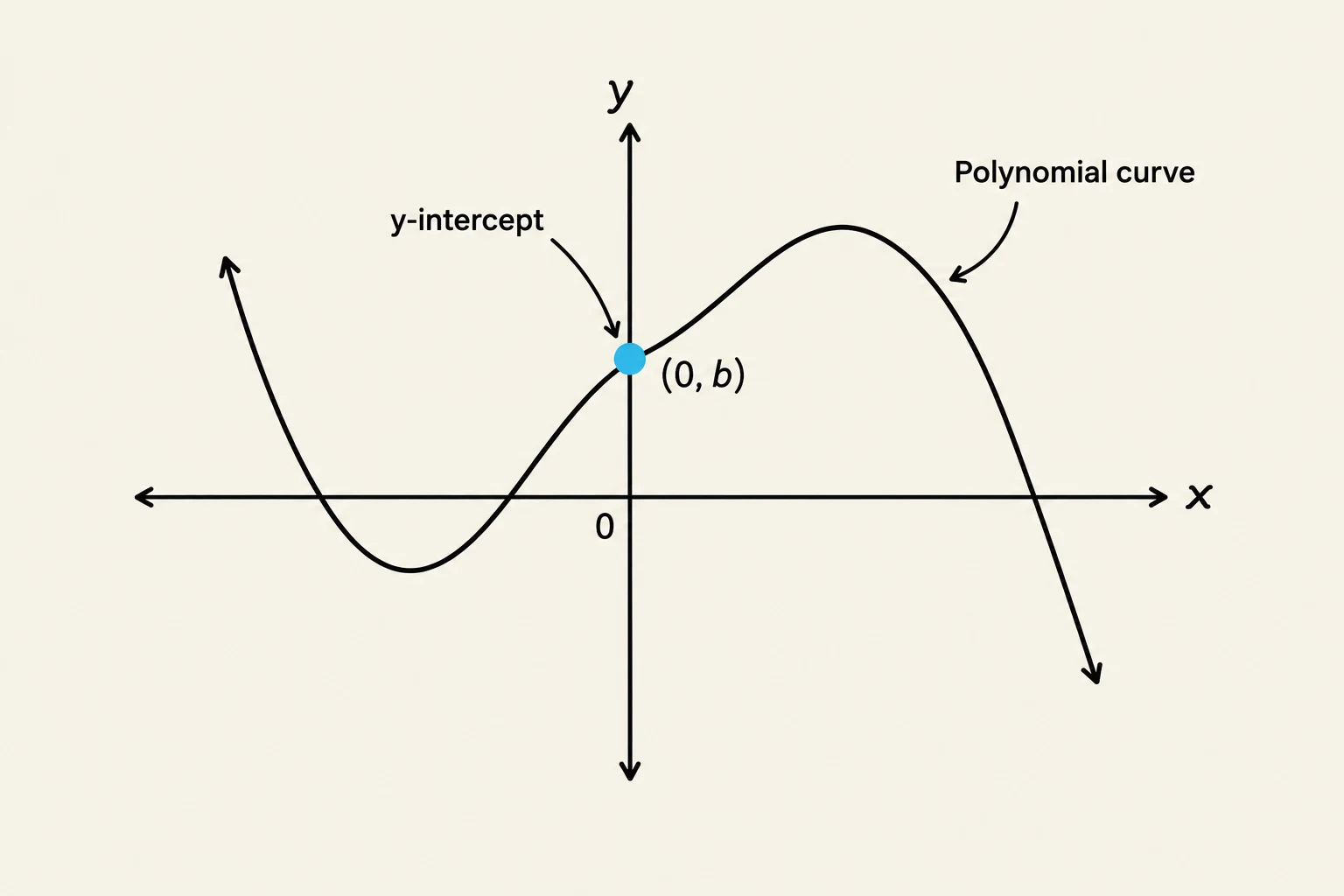
The vertical intercept, or y-intercept, is the point where the graph crosses the y-axis. At this point, the value of x is always zero. To find it, simply plug 0 in for x and solve for f(x).
Horizontal Intercepts (x-intercepts)
The horizontal intercepts, or x-intercepts, are the points where the graph meets the x-axis. At these points, the value of y (or f(x)) is zero. To find them, set f(x)=0 and solve for x. These values are often referred to as the "zeros" or "roots" of the polynomial.
A graph illustrating a polynomial curve with its y-intercept labeled at (0, b).
Multiplicity and Graphical Behavior
Once you have identified your x-intercepts, you must determine how the graph behaves at each one. This behavior is dictated by the multiplicity of the intercept.
Multiplicity refers to the number of times a specific factor appears in the factored form of the polynomial. If a polynomial has a factor (x−h)p, then h is an x-intercept with a multiplicity of p.
The value of the exponent p determines the shape of the graph near the intercept (h,0):
Multiplicity of 1 (p=1): The graph passes straight through the x-axis like a line.
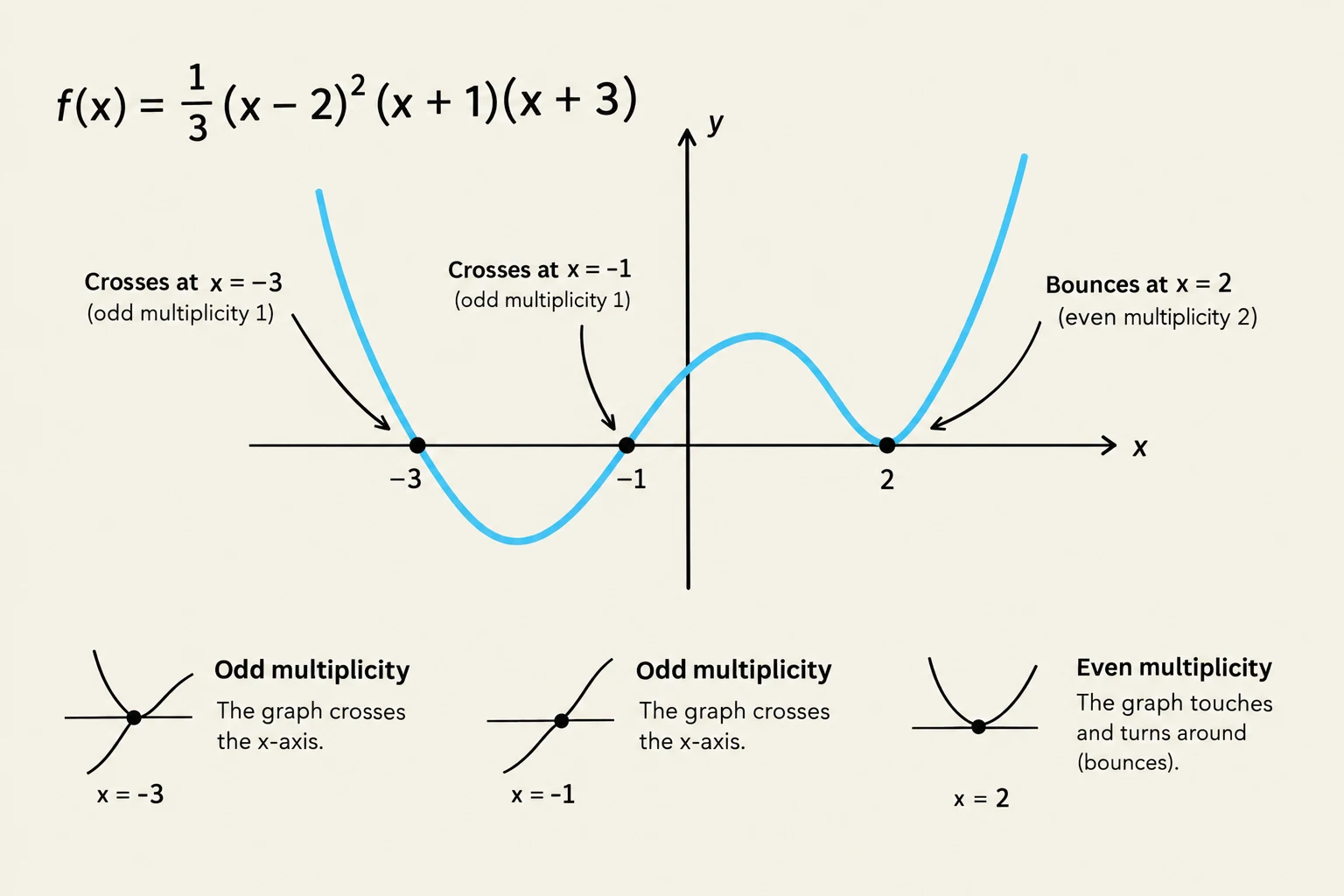
Even Multiplicity (p=2,4,…): The graph touches the x-axis and "bounces" back in the direction it came from, behaving like a parabola at that point.
Odd Multiplicity greater than 1 (p=3,5,…): The graph passes through the x-axis but "flattens out" as it crosses, creating an S-shaped inflection point.
Graphs illustrating the behavior of functions at x=a based on their multiplicity: multiplicity 1 crosses the x-axis, multiplicity 2 touches and turns around, and multiplicity 3 flattens at the x-axis before crossing.
Exam Tip: When looking at a factored equation, always check the exponents on each factor. These exponents are your multiplicities and will tell you exactly whether to "cross" or "bounce" at each intercept.
Polynomial Sketching: A Step-by-Step Guide
To create a complete sketch of a polynomial, you should combine several pieces of information into a single cohesive shape. Follow this checklist:
End Behavior (Long Run Behavior): Determine where the graph goes as x approaches infinity or negative infinity.
Turning Points: Note that a polynomial of degree n can have at most n−1 turning points.
y-intercept: Locate the point (0,y).
x-intercepts and Multiplicities: Plot the zeros and decide if the graph crosses or bounces at each.
Worked Example: Building a Polynomial from Scratch
Sometimes, you are asked to do the reverse: write an equation based on a given graph or set of characteristics.
Problem: Find a polynomial of degree 4 with:
x-intercepts at (2,0) with multiplicity 2.
x-intercepts at (−1,0) and (−3,0) with multiplicity 1.
A y-intercept at (0,4).
Step 1: Set up the factored form
Using the intercepts and multiplicities, we write the factors. Remember that for an intercept h, the factor is (x−h).
For x=2 (mult 2): (x−2)2
For x=−1 (mult 1): (x−(−1))→(x+1)
For x=−3 (mult 1): (x−(−3))→(x+3)
We include a leading coefficient a because we don't yet know the vertical stretch:
f(x)=a(x−2)2(x+1)(x+3)
Step 2: Solve for a using the y-intercept
We know that when x=0, f(x)=4. Plug these values into our equation:
This graph illustrates the behavior of a polynomial function at its roots, distinguishing between odd and even multiplicities. Odd multiplicities result in the graph crossing the x-axis, while even multiplicities cause the graph to touch and turn around (bounce) at the x-axis.
By following these steps—identifying intercepts, determining multiplicity, and checking end behavior—you can master the art of sketching any polynomial function.
Keep reading for free.
Create an account to finish this reading and make it part of your study routine.