An introduction to data visualization techniques in biostatistics, covering data types, bar graphs, histograms, and box plots for representing and analyzing data distributions.
In biostatistics, data visualization is much more than just creating "pretty pictures." It is a fundamental process used to represent relationships, distributions, and patterns within datasets effectively. Because biological data can vary wildly in nature—ranging from the number of children in a household to the precise height of a patient—the choice of a graphic method depends primarily on the type of data being analyzed.
Understanding Data Types
Before selecting a graph, a researcher must identify the scale of measurement of their variables. Variables are characteristics that change from subject to subject, while an observation is a specific measured value of that variable.
There are two primary categories of quantitative data:
Discrete Data: These are numeric values that represent countable quantities, such as the number of children in a family (e.g., 0, 1, 2...).
Continuous Data: These are numeric values that can take any value within a range, such as height or financial profit.
Additionally, we often deal with categorical data (or qualitative data), which represents non-numeric groups, such as a person's country of origin or employment status.
Representing Groups: Bar Graphs and Histograms
Once the data type is identified, we can choose the appropriate tool for visualization.
Bar Graphs for Categorical and Discrete Data
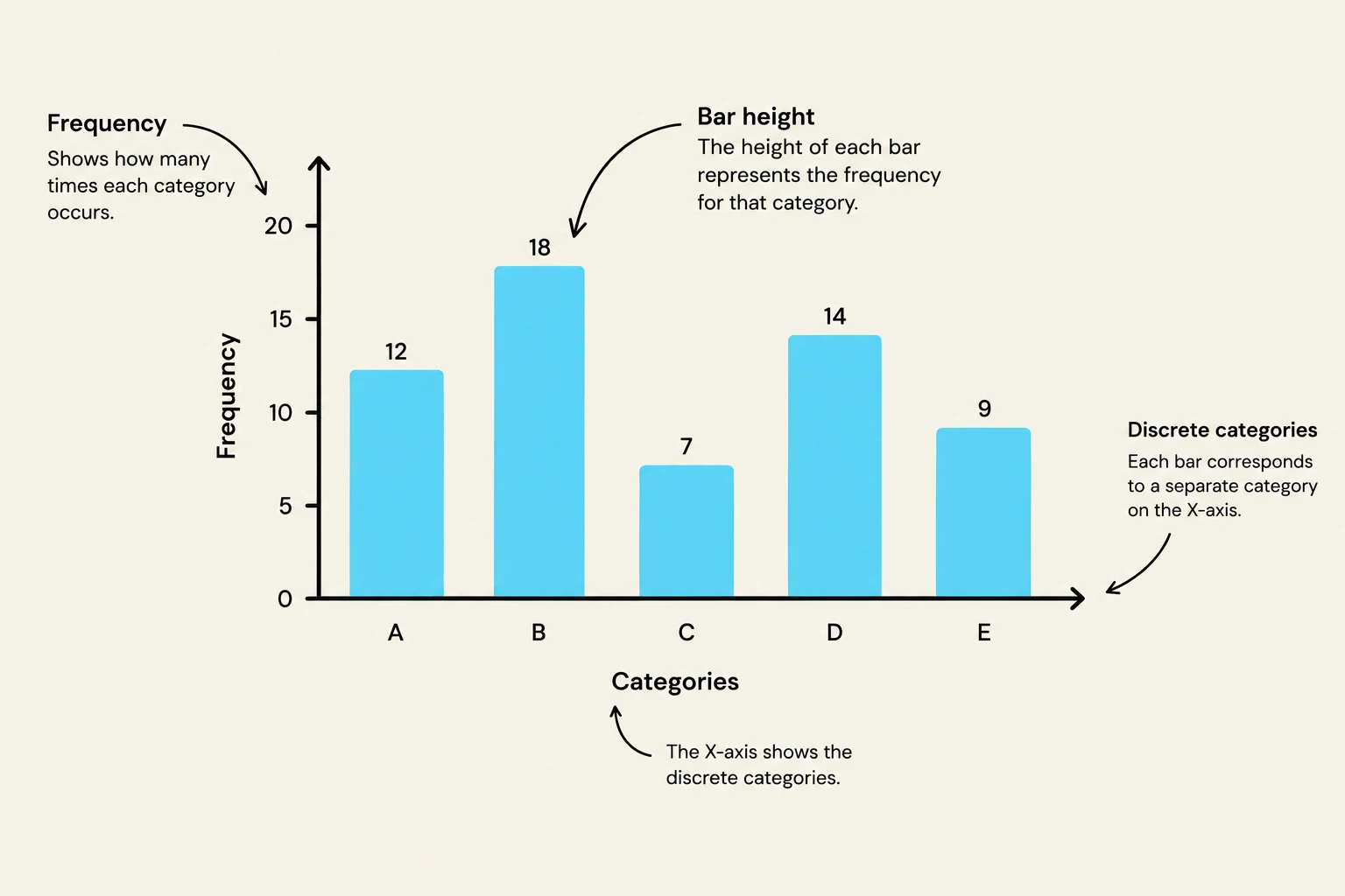
When working with categorical or discrete data, the bar graph is the standard choice. In a bar graph, each bar represents a specific group or category, and the height of the bar indicates the frequency—the number of times that specific value or category occurs in the dataset.
A bar chart illustrating frequency distribution across discrete categories, with labels explaining the axes and bar height representation.
Histograms for Continuous Data
For continuous data, we use a histogram. While they look similar to bar graphs, histograms are used to show the distribution of values across continuous intervals (bins) rather than distinct categories. This allows researchers to see the "shape" of the data, such as where most values cluster.
Analyzing Distribution: The Box Plot
One of the most powerful tools in a biostatistician's arsenal is the box plot. Unlike bar graphs or histograms, box plots are uniquely suited for comparing continuous data across different categorical groups.
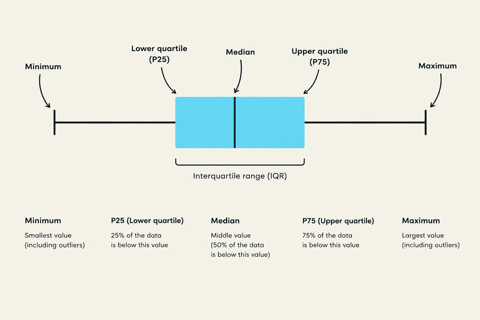
A box plot provides a visual summary of the data's distribution and skewness (the asymmetry of the distribution) by illustrating the relationship between several key measures of location:
Median: The middle value of the dataset when ordered from smallest to largest.
Upper Quartile (P75): The 75th percentile, marking the point below which 75% of the data falls.
Lower Quartile (P25): The 25th percentile, marking the point below which 25% of the data falls.
The "box" itself represents the Interquartile Range (IQR), which contains the middle 50% of the data. Vertical lines, often called "whiskers," extend from the P75 to the largest non-outlying value and from the P25 to the smallest non-outlying value.
A box plot illustrating statistical measures including minimum, lower quartile (P25), median, upper quartile (P75), and maximum, along with the interquartile range (IQR).
Identifying Outliers
A box plot is also essential for identifying outlying values—data points that fall significantly far from the rest of the distribution. Mathematically, an observation X is considered an outlier if it meets either of the following criteria:
XX>P75+1.5×(P75−P25)<P25−1.5×(P75−P25)
Exam Tip: When describing a distribution, remember that the median and IQR are often paired together because both are based on the order of observations rather than just the values, making them more robust against outliers than the mean and standard deviation.
The Ethics of Visualization
A graphic is only useful if it is clear and honest. To ensure the integrity of a scientific figure, several components must be present:
Labeled X- and Y-axes: Both axes must be clearly named.
Units of Measurement: It is vital to indicate whether you are measuring lbs, meters, or counts.
Tick Marks: Appropriate intervals on the axes to allow for reading values.
Descriptive Title: A title that provides sufficient detail to understand the context.
Key or Legend: Necessary to distinguish between different colors, shapes, or data series.
Full Acronyms: Avoid ambiguity by spelling out all acronyms.
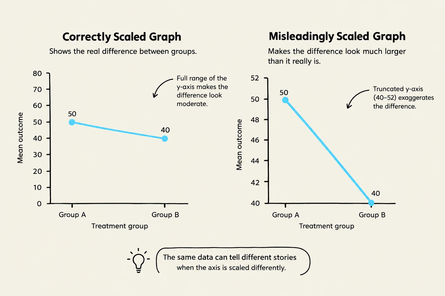
Biostatisticians have an ethical responsibility to represent data accurately. Misleading scales or improper axis configurations can create false impressions. For example, a poorly scaled Y-axis might suggest a consistent decline in a trend (such as COVID-19 cases) when the data does not actually support such a conclusion. Proper visualization requires careful consideration of how data points are plotted in relation to the axes to avoid misinterpretation.
This illustration demonstrates how scaling of the y-axis in a graph can alter the perception of data, showing a moderate difference with a full y-axis range and an exaggerated difference with a truncated y-axis.
Keep reading for free.
Create an account to finish this reading and make it part of your study routine.