An explanation of economic elasticity, including price elasticity of demand and supply, their determinants, and applications in understanding market behavior and revenue.
In economics, knowing that a change in price will affect the quantity of a good sold is only the first step. To make informed decisions, businesses and policymakers need to know how much that quantity will change. This is where the concept of elasticity comes in. Elasticity serves as a measure of the responsiveness of quantity demanded or quantity supplied to one of its determinants, such as price, income, or the prices of related goods. By quantifying these responses, elasticity allows us to predict how markets will react to various economic events.
Understanding Elasticity
At its core, elasticity measures sensitivity. If a small change in a determinant (like price) leads to a massive change in behavior (like quantity demanded), we say the relationship is "elastic." If the change in behavior is minimal, the relationship is "inelastic".
There are several primary types of elasticity:
Demand Elasticities: These include Price Elasticity of Demand, Income Elasticity, and Cross-Price Elasticity.
Supply Elasticity: Specifically, the Price Elasticity of Supply.
Price Elasticity of Demand
The most common application is the Price Elasticity of Demand, which measures the percentage change in quantity demanded in response to a 1 percent change in price.
To calculate this, we use the following formula:
Price elasticity of demand=%ΔP%ΔQ
Where %ΔQ represents the percentage change in quantity demanded and %ΔP represents the percentage change in price.
Because price and quantity demanded always move in opposite directions (the Law of Demand), the resulting calculation will yield a negative number. However, for the sake of simplicity in analysis, economists often use the absolute value of the result.
Worked Example: The Book Market
Suppose a 10% increase in the price of books leads to a 30% decrease in the quantity demanded. We calculate the elasticity as follows:
Elasticity=10%−30%=−3
In this scenario, the change in quantity is three times the change in price. This means that for every 1% increase in price, the quantity demanded will drop by 3%.
A graph illustrating a steep demand curve, which signifies low elasticity, meaning demand is less responsive to price changes. It shows that a small change in price leads to a relatively small change in quantity demanded.
Classifying Demand Types
We can categorize demand based on the magnitude of the response:
Inelastic Demand: The absolute value of the percentage change in quantity is less than the percentage change in price (∣%ΔQ∣<∣%ΔP∣). A perfectly inelastic demand is represented by a vertical line, where quantity remains fixed regardless of price.
Elastic Demand: The absolute value of the percentage change in quantity is greater than the percentage change in price (∣%ΔQ∣>∣%ΔP∣). A perfectly elastic demand is represented by a horizontal line, where price is fixed.
Unitary Elastic Demand: The percentage changes are equal (∣%ΔQ∣=∣%ΔP∣).
Exam Tip: Remember that elasticity is NOT the same as the slope of the demand curve. While they are related, a linear demand curve has a constant slope but can take on all possible elasticity values at different points along the curve.
Determinants of Price Elasticity of Demand
Why are some goods more sensitive to price changes than others? Several factors determine how elastic a demand curve will be:
Availability of Substitutes: This is a major driver. If more substitutes are available, demand becomes more elastic because consumers can easily switch to another product.
Necessities versus Luxuries: Necessities tend to have more inelastic demand, while luxuries tend to have more elastic demand.
Definition of the Market: Narrowly defined markets (e.g., a specific brand of vanilla ice cream) have more elastic demand than broadly defined markets (e.g., food in general).
Consumers’ Willingness to Search: When consumers are more willing to search for low-cost alternatives, demand becomes more elastic.
Time Horizon: The longer the time horizon, the more elastic the demand tends to be.
Calculating Elasticity: The Midpoint Method
A common issue when calculating elasticity using a standard percentage change formula is that the result changes depending on whether you are moving from point A to B or B to A. To solve this, economists use the Midpoint Method.
The formula for the midpoint method is:
Elasticity=(P1+P2)/2ΔP(Q1+Q2)/2ΔQ
For example, if a pizza restaurant raises its price from $$9$to$$11$ and the quantity sold falls from 55 to 45 per day, the midpoint method ensures a consistent calculation regardless of the direction of the price change.
Applications of Elasticity
Total Revenue and Price Changes
Price elasticity of demand helps predict how price changes will affect Total Revenue (TR), where TR=P×Q. Because price and quantity move in opposite directions, the effect on revenue depends on which change is proportionally larger:
Unitary Elastic: If price increases by 1% and quantity drops by 1%, TR remains unchanged.
Elastic Demand: If price increases by 1% and quantity drops by more than 1%, TR will fall.
Inelastic Demand: If price increases by 1% and quantity drops by less than 1%, TR will increase.
This illustration displays three types of demand curves: perfectly elastic, perfectly inelastic, and normal (downward sloping), along with explanations of how price changes affect quantity demanded in each case.
Other Types of Elasticity
Beyond price, we also measure:
Income Elasticity of Demand: The percentage change in quantity in response to a 1% change in income.
Normal Goods: Have positive income elasticity.
Inferior Goods: Have negative income elasticity.
Cross-Price Elasticity of Demand: The percentage change in quantity of one good in response to a 1% change in the price of another good.
Substitutes: Have positive cross-price elasticity.
Complements: Have negative cross-price elasticity.
Price Elasticity of Supply
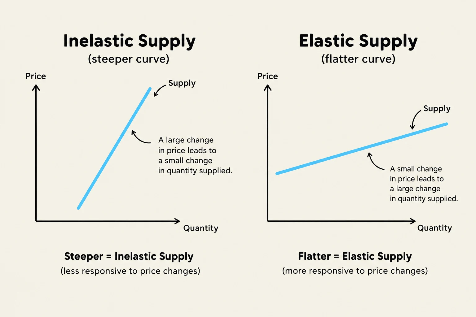
Finally, we consider the Price Elasticity of Supply, which is the percentage change in quantity supplied in response to a 1 percent change in price. Like demand, supply can be elastic (quantity change is more than proportional to price change) or inelastic (quantity change is less than proportional to price change).
The steepness of the supply curve reflects its elasticity: the steeper the curve, the more inelastic the supply.
Determinants of Supply Elasticity include:
The possibility of holding inventories (storable goods are more elastic).
Availability of inputs and idle capacity.
Ease of entry or exit into the market.
The time horizon (longer time horizons allow for more elastic supply).
This image illustrates the concepts of inelastic and elastic supply using supply and demand graphs. Inelastic supply, represented by a steeper curve, indicates that a large change in price leads to a small change in quantity supplied. Elastic supply, shown by a flatter curve, signifies that a small change in price leads to a large change in quantity supplied. The graphs demonstrate that steeper curves are less responsive to price changes, while flatter curves are more responsive.
Keep reading for free.
Create an account to finish this reading and make it part of your study routine.