Explore the fundamental types of mathematical functions, including linear, exponential, power, trigonometric, and logarithmic functions. Learn analytical techniques for describing their movement and shape, including graphical identification, approximation, and asymptotic behavior.
Understanding the behavior of mathematical functions is a cornerstone of calculus. Rather than simply memorizing formulas, mathematicians focus on how functions grow, how they behave near specific points, and how they appear when plotted on a coordinate plane. This article explores the fundamental types of functions and the analytical techniques used to describe their movement and shape.
This illustration compares a linear function (y=2x) with a constant difference of +2 in its y-values for each unit increase in x, to an exponential function (y=2^x) with a constant ratio of x2 in its y-values for each unit increase in x.
Core Function Types
To analyze a function, one must first identify its algebraic form. Different families of functions exhibit distinct patterns in their data and graphs.
Linear Functions
Linear functions follow the form $y = mx + b$, where m is the slope and b is the y-intercept. A defining characteristic of linear functions is that they exhibit constant differences. If you look at a table of values where the x-values increase by equal increments, the corresponding y-values will also change by a constant amount.
Exponential Functions
Exponential functions take forms such as y=a⋅nx or y=aekx. Unlike linear functions, exponential functions are characterized by constant ratios. In a data table, for equal increments of x, the y-values are multiplied by a consistent factor. These functions can represent rapid growth (when the base is greater than 1) or rapid decay (when the base is between 0 and 1).
Power Functions
Power functions are expressed as f(x)=xn. These are essential for understanding polynomial behavior. For example:
f(x)=xn increases steeply for large x if n>1.
f(x)=x−n (where n>1) decreases as x becomes large.
f(x)=x1/n (root functions) grows more slowly than higher-degree power functions.
Trigonometric and Logarithmic Functions
Trigonometric functions like sin(x), cos(x), and tan(x) introduce periodicity into analysis. Logarithmic functions, specifically log(x), are the inverses of exponential functions.
Mathematical Notation Tip: In higher-level mathematics, log(x) typically denotes the natural logarithm (ln(x)), rather than the base-10 logarithm used in some introductory contexts.
Graphical Analysis and Identification
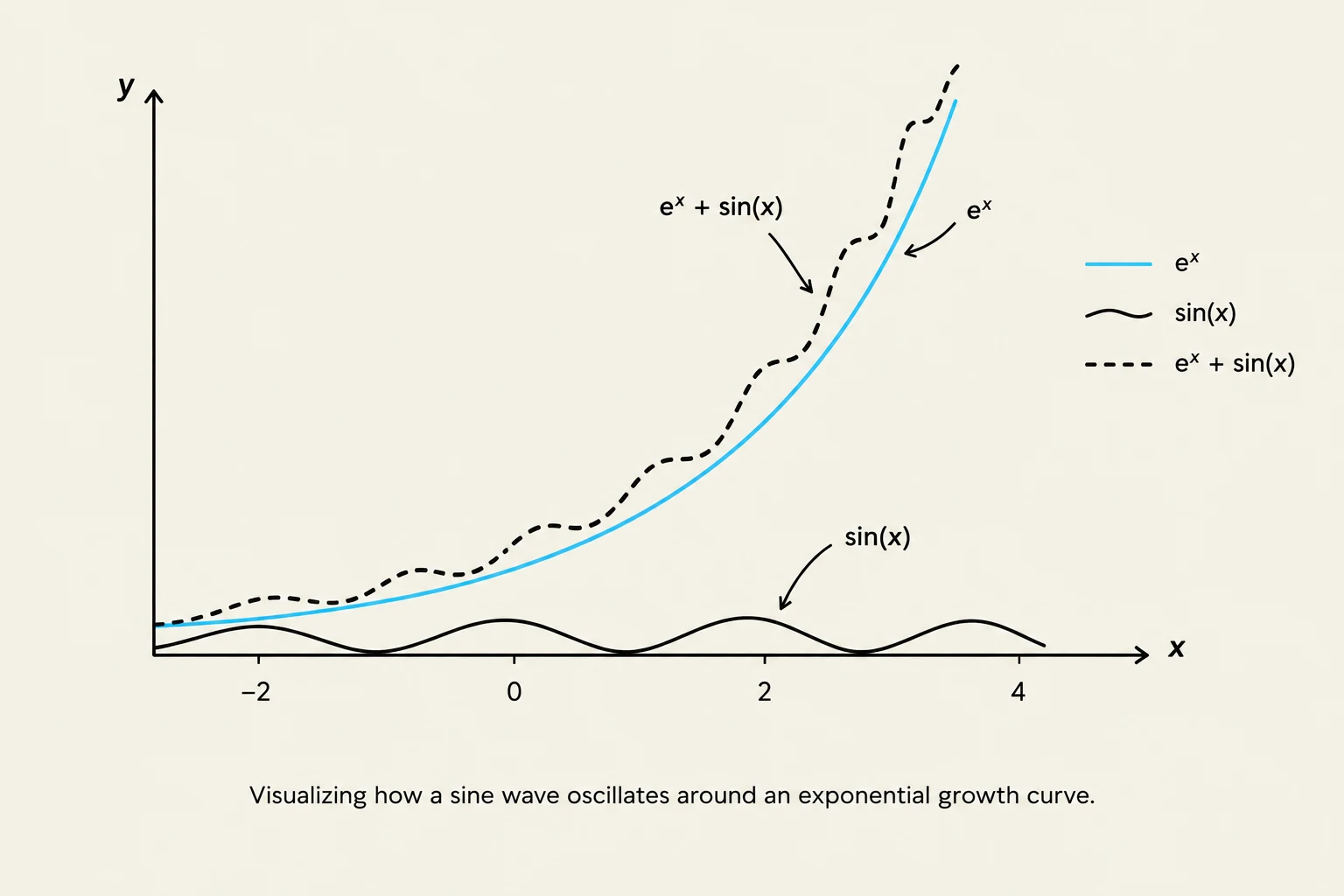
Visualizing how a sine wave oscillates around an exponential growth curve.
A key skill in calculus is "matching" an equation to its visual representation on the xy plane. This requires recognizing standard curves such as x2 (parabolas), 1/x (hyperbolas), x, and ∣x∣ (V-shaped graphs).
When dealing with complex combinations, such as g(x)=sin(x)+ex, you should analyze the component functions to predict the result. For instance, the exponential term ex will dominate the overall growth for large x, while the sin(x) term will cause small oscillations around that growth path.
Function Approximation and Dominance
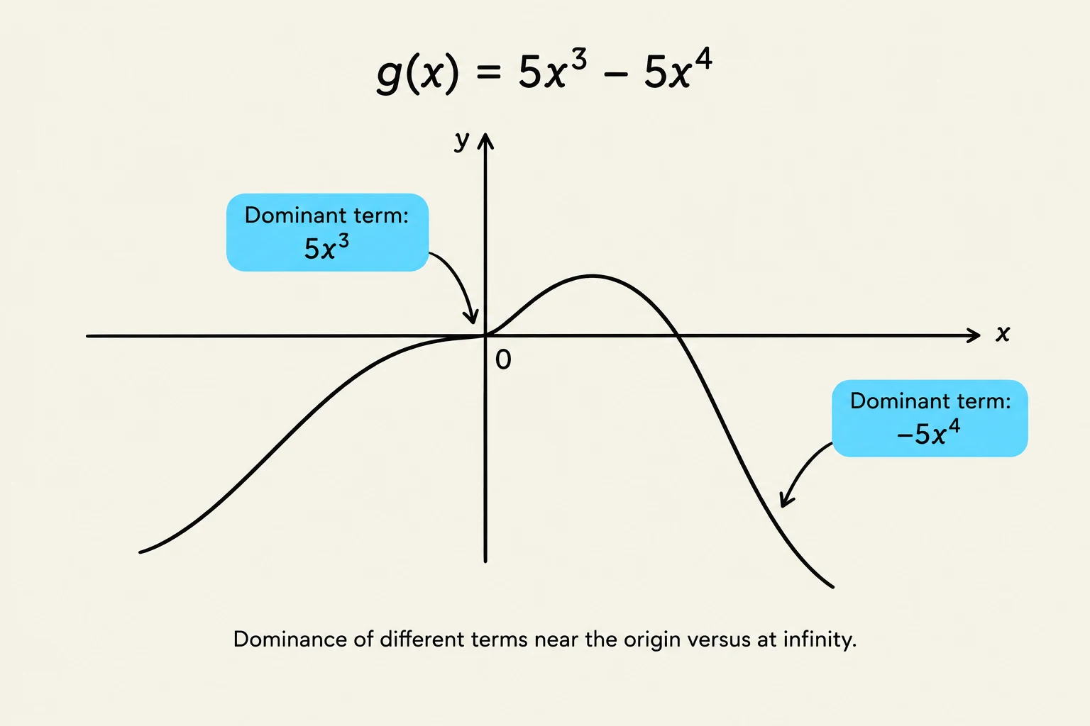
A graph illustrating the dominance of terms in the function g(x) = 5x^3 - 5x^4 near the origin and at infinity.
One of the most powerful tools in function analysis is the concept of dominance. When a function is composed of several terms, different terms "take control" depending on the value of x.
Behavior Near the Origin (Small x)
When x is very close to zero, the term with the lowest degree (the smallest exponent) dominates the function's behavior. For example, in the function g(x)=5x3−5x4, the x3 term is much larger than the x4 term when x is a tiny fraction (like 0.01). Therefore, near the origin, g(x)≈5x3.
Behavior Far From the Origin (Large x)
As x becomes very large, the term with the highest degree dominates. Using the same example, g(x)=5x3−5x4, the x4 term grows much faster than the x3 term as x→∞. Thus, for large x, the function behaves like −5x4.
By identifying these dominant terms, we can approximate complex functions using simple power functions xp for small x and xq for large x.
Asymptotic Behavior and Limits
As we move toward the study of limits, we focus on how functions approach specific values or boundaries.
Sign Analysis
It is often necessary to determine if a function is positive, negative, or neither as x approaches a certain value. For example, when analyzing f(x)=x6+x4−x3 for very small positive x, the x3 term is the most significant. Since −x3 will be negative for small positive x, the function's sign will be negative.
Physical and Biological Models
Function analysis is used to model real-world phenomena:
Physics: Forces can be modeled by power functions. An attractive force might be inversely proportional to r3 (α/r3), while a repulsive force might be inversely proportional to r2 (β/r2).
Biology: The "squashing function" or "threshold function," y=1+eax+b1, is used to model how regulatory genes respond to inputs, creating a smooth transition between "off" and "on" states.
Exam Tip: When matching graphs to equations, always check the "end behavior" (what happens as x→∞) and the "intercepts" (what happens at x=0) to quickly eliminate incorrect choices.
Keep reading for free.
Create an account to finish this reading and make it part of your study routine.