Economic Data and Index Numbers: Measuring and Visualizing the Economy
This article explores how economists use index numbers to measure relative changes in variables over time, such as the Consumer Price Index (CPI), and how they organize and visualize economic data using cross-sectional data, time-series data, and scatter diagrams to understand correlations.
In the study of economics, data serves as the essential bridge between abstract theory and real-world reality. While theories provide a framework for understanding how variables interact, economists rely on empirical observations to test whether those theories hold true. To make sense of the vast amount of information generated by markets, governments, and households, economists use specific tools to summarize, compare, and visualize data. This article explores how we measure changes over time using index numbers and how we organize different types of economic information through various graphing methods.
Understanding Index Numbers
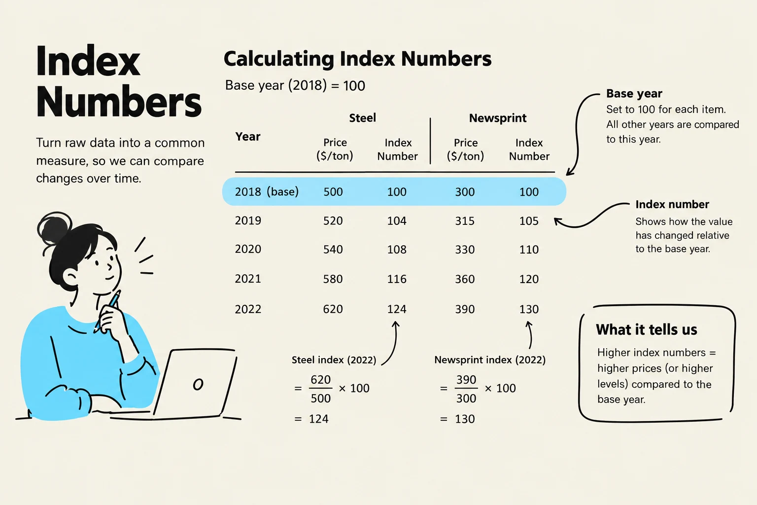
An index number is a statistical tool used to measure the relative change in a variable over time or across different categories. Rather than looking at raw numbers, which can be difficult to compare if they are of different scales, index numbers express values relative to a specific reference point known as the base period.
In the base period, the index is conventionally assigned a value of 100. By setting this benchmark, we can easily see how much a variable has increased or decreased compared to that starting point.
The Calculation Formula
To calculate an index number for a given period, you divide the absolute value of the variable in that period by the absolute value in the base period, and then multiply by 100:
Index Number=(Absolute value in base periodAbsolute value in given period)⋅100
Example Walkthrough:
Suppose we are tracking the output of steel. If the output in our base year (2014) was 200 units and the output in 2024 is 245 units, the calculation would be:
(200245)⋅100=122.5
This tells us that steel output in 2024 is 22.5% greater than it was in the base year.
This illustration explains how to calculate index numbers using steel and newsprint prices as examples, with 2018 as the base year. It shows how index numbers reflect changes relative to the base year and what higher index numbers signify.
The Consumer Price Index (CPI)
The most widely recognized application of index numbers is the Consumer Price Index (CPI). The CPI measures the average price that consumers pay for a typical "basket" of goods and services.
Because the CPI tracks the cost of living, it is a vital indicator for understanding inflation. When the CPI rises, it indicates that the purchasing power of money is decreasing, as consumers must spend more to acquire the same basket of goods. Governments and central banks monitor the CPI closely to make decisions regarding monetary policy and interest rates.
Organizing Economic Data
When economists collect information, they generally categorize it into two distinct formats based on how the observations are structured: cross-sectional data and time-series data.
Cross-Sectional Data
Cross-sectional data involves observations taken at a single point in time across many different units. For example, if an economist wants to compare the average house prices across all ten Canadian provinces in the year 2024, they are using cross-sectional data. This allows for comparisons between different entities (like provinces, companies, or individuals) at one specific moment.
Time-Series Data
In contrast, time-series data tracks a single variable over a sequence of time intervals. An example would be tracking the Canadian unemployment rate every month from 1978 to 2024. This format is essential for identifying trends, cycles, and long-term shifts in the economy.
A line graph illustrating Canada's unemployment rate from 1978 to 2024, highlighting significant economic events such as the early 1980s recession, the 2007 low point, the global financial crisis, and the pandemic spike in 2020.
Visualizing Relationships: The Scatter Diagram
While cross-sectional and time-series data help us organize information, we often need to see how two different variables relate to one another. This is where the scatter diagram becomes useful.
A scatter diagram is a graph that displays two variables, with one measured on the horizontal axis (X) and the other on the vertical axis (Y). Each point on the graph represents a single observation where the X and Y values for that specific unit are plotted together.
Correlation and Causality
By looking at the pattern of dots in a scatter diagram, economists can identify correlations:
Positive Correlation: The points generally move upward from left to right, meaning X and Y move in the same direction.
Negative Correlation: The points move downward from left to right, meaning X and Y move in opposite directions.
Important Distinction: A scatter diagram can show that two variables are correlated, but it does not prove causality. Just because X and Y move together does not mean that X causes Y to happen. Establishing causality often requires much more advanced statistical techniques, such as randomized controlled trials.
This scatter plot illustrates the relationship between investment in billions of USD and GDP growth rate in percentage. The upward trend indicates a positive correlation, suggesting that higher investment is generally associated with higher GDP growth.
Summary Table of Data Types
Data Type
Focus
Example
Cross-Sectional
Comparison across entities at one time
House prices in different provinces in 2024
Time-Series
Change in one entity over time
Monthly unemployment rates from 1978–2024
Index Numbers
Relative change compared to a base
Consumer Price Index (CPI)
By mastering these methods of measurement and visualization, economists can move from simply observing "what is" to building and testing the complex theories that explain how the world works.
Keep reading for free.
Create an account to finish this reading and make it part of your study routine.