Descriptive Statistics and Measures of Variability
An introduction to descriptive statistics, including measures of central tendency (mean, median, mode) and measures of variability (range, standard deviation, relative variation).
When we collect data, we are often faced with a massive collection of numbers that, on their own, tell us very little. To make sense of this information, we use descriptive statistics. Descriptive statistics are tools used to summarize, organize, and simplify data so that we can understand its core characteristics. While inferential statistics aim to make predictions about a larger population based on a sample, descriptive statistics focus on describing what is actually present in the data set at hand.
Measures of Central Tendency
The first step in describing a dataset is finding its "center." This is typically done using three primary measures: the mean, the median, and the mode.
The Mean
The mean is the arithmetic average of a dataset. It is calculated by summing all the values in a set and dividing by the total number of observations. For example, if a police lieutenant reviews the number of traffic citations issued per day by 10 officers and finds the total is 220, the mean is:
10220=22.0
The Median
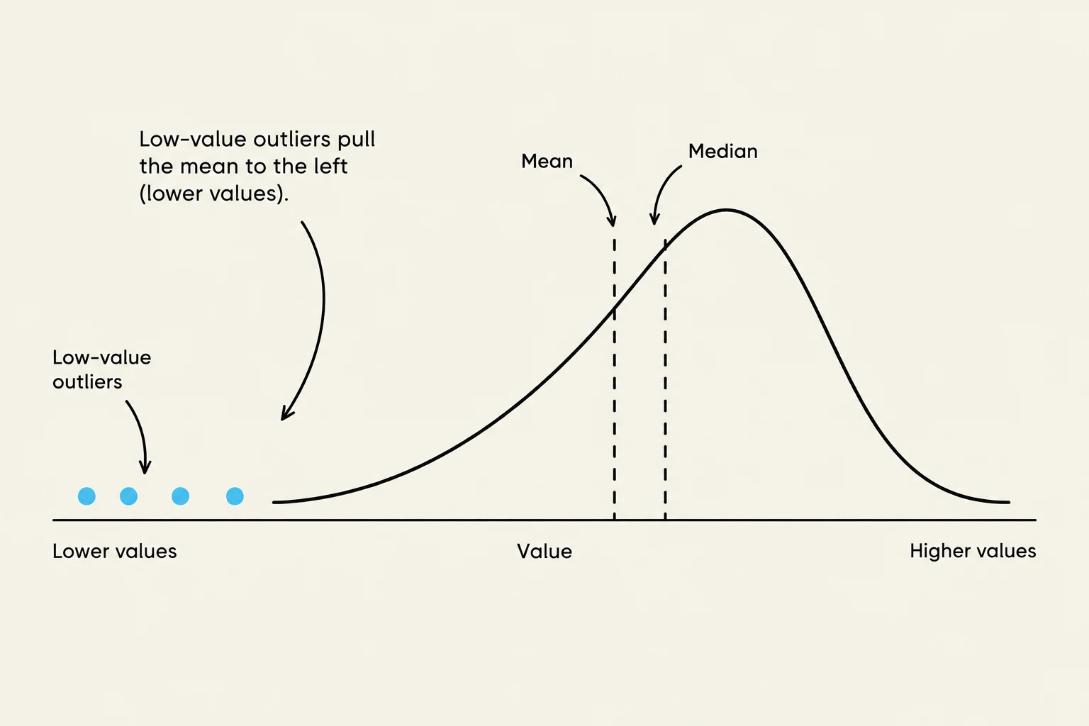
The median is the middle value when the data points are arranged in ascending or descending order. If there is an even number of observations, the median is the average of the two middle values. A critical property of the median is its resistance to outliers—extreme values that are significantly higher or lower than the rest of the data. Because the mean incorporates every value into its calculation, a single massive outlier can pull the mean away from the center, whereas the median remains stable.
The Mode
The mode is the value that appears most frequently in a dataset. A dataset can have one mode, multiple modes, or no mode at all if every value is unique.
Exam Tip: If you are told that the mean of a sample is lower than the median, this suggests the distribution is "skewed to the left" or negatively skewed.
A diagram illustrating how low-value outliers skew the mean to the left in a distribution.
Percentiles and Quartiles
Beyond the center, we often want to know where a specific value stands in relation to the rest of the group. This is where percentiles come in.
A percentile is a measure indicating the value below which a given percentage of observations fall. For instance, the 75th percentile is the value that is greater than 75% of the data.
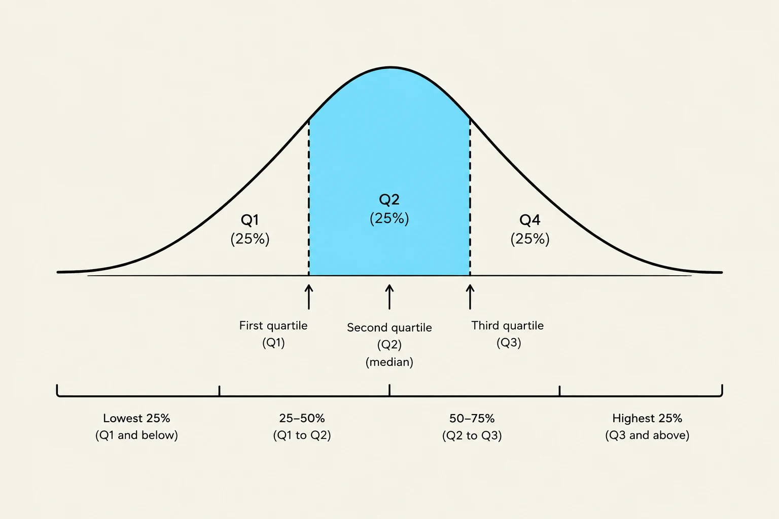
To make these measurements more manageable, we divide the data into four equal parts called quartiles:
First Quartile (Q1): The 25th percentile; it marks the point below which 25% of the data falls.
Second Quartile (Q2): This is identical to the median.
Third Quartile (Q3): The 75th percentile; it marks the point below which 75% of the data falls.
A diagram illustrating quartiles and their distribution on a bell curve, showing Q1, Q2 (median), and Q4, each representing 25% of the data.
Measures of Variability
Knowing the average is rarely enough. To understand the "spread" or "scatter" of the data, we must use measures of variability. These measures describe how much the data values deviate from the center and from each other.
Range and Standard Deviation
The simplest measure of spread is the range, which is the difference between the highest and lowest values in a set. However, the range is highly sensitive to outliers.
A more sophisticated measure is the standard deviation. This tells us how much, on average, the data points deviate from the mean. A low standard deviation indicates that the data points tend to be close to the mean, while a high standard deviation indicates that the data are spread out over a wider range of values.
Relative Variation
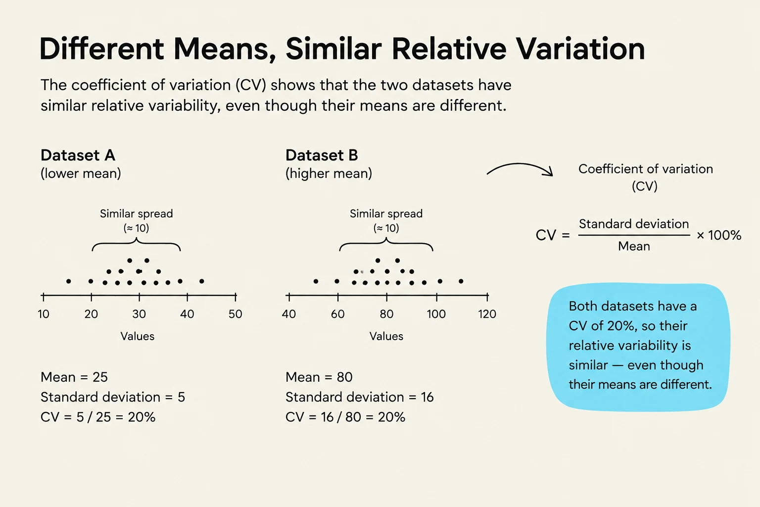
Sometimes, comparing the standard deviation of two different datasets is like comparing apples to oranges—especially if they have different scales (for example, comparing the sales of a small boutique to a massive supermarket). In these cases, we use relative variation (often expressed as the coefficient of variation). This allows us to compare the dispersion of two datasets relative to their means, providing a "fairer" comparison of volatility or spread.
This illustration explains the concept of the coefficient of variation (CV) using two datasets with different means but similar relative variation. It shows how to calculate CV and provides an example demonstrating that datasets with different absolute values can have the same relative variability.
Practical Application: Growth Rates
In business and economics, we often look at the average annual increase over time. If sales increase by different percentages each year (e.g., 10%, 8%, 6%, and 4%), calculating the average requires careful attention to how these rates compound or average out over the period.
Summary Table of Key Terms
Term
Definition
Sensitivity to Outliers
Mean
Arithmetic average
High
Median
Middle value
Low
Mode
Most frequent value
Low
Standard Deviation
Average distance from the mean
High
Range
Difference between Max and Min
Very High
By combining measures of central tendency with measures of variability, researchers can build a complete picture of any dataset, moving from a simple list of numbers to meaningful, actionable insights.
Keep reading for free.
Create an account to finish this reading and make it part of your study routine.