Describing Data and Statistical Measures in Econometrics
Learn how to describe data in econometrics by classifying variables, calculating central tendencies (mean, median, mode), measuring variability (range, variance, standard deviation, IQR), and examining relationships between variables (covariance, correlation, elasticity). Includes visualizations like histograms and sca
In the field of econometrics, the first step toward understanding economic relationships is gathering and describing data. Before we can estimate complex models or test theories, we must be able to summarize the information we have collected. Describing data involves classifying variables, calculating central tendencies, measuring how much data points vary, and examining how two variables move together.
Data Classification and Visualization
To describe data effectively, we must first identify the type of variable we are dealing with. Variables are generally categorized into two groups:
Qualitative (Categorical) Data: These are observations that fall into specific categories or labels. The values are not numbers in a mathematical sense; for example, "industry of employment" or "region" are labels where arithmetic (like adding two regions) makes no sense.
Quantitative (Numerical) Data: These are observations expressed as numbers where arithmetic operations are meaningful. Quantitative data can be further divided:
Discrete: The variable can only take a countable list of values (e.g., number of children).
Continuous: The variable can take any value within an interval (e.g., hourly wage).
Visualizing Categorical Data
For qualitative data, we often use a frequency table to show the count (fj) or the relative frequency (fj/n) of each category. These are visualized using:
Bar Charts: One bar is drawn per category, with the height representing the frequency or relative frequency.
Pie Charts: One slice is drawn per category, with the area representing the relative frequency.
Visualizing Quantitative Data
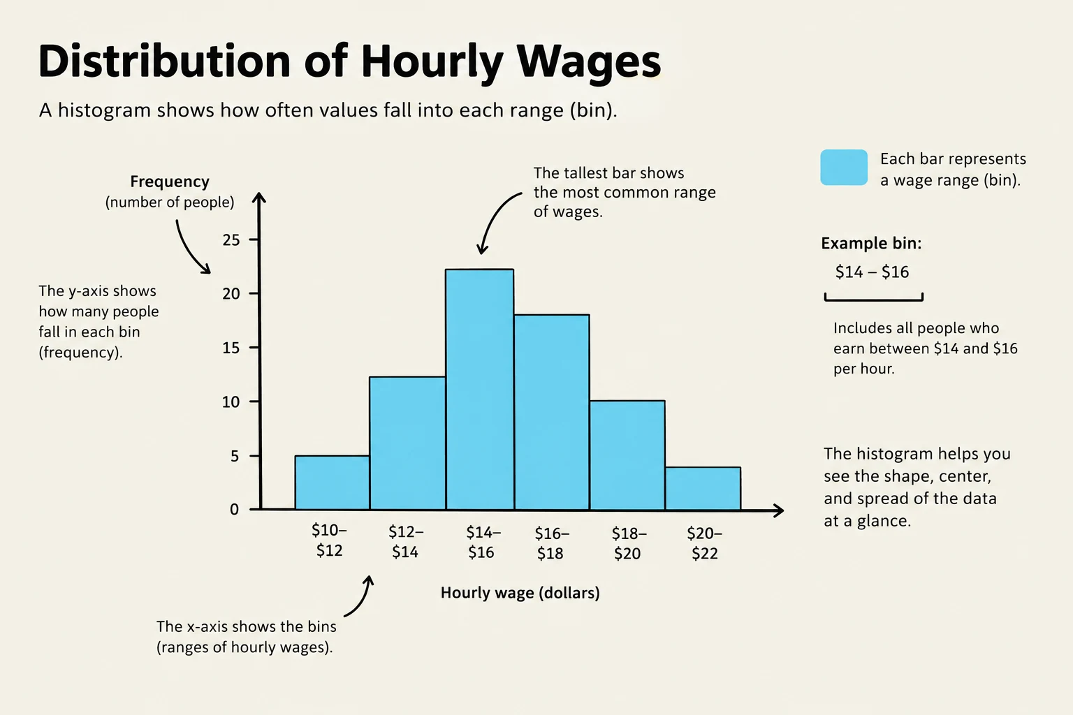
Because continuous variables like wages can have hundreds of distinct values, we use a histogram. We split the range of the variable into bins (adjacent intervals of equal width) and count how many observations fall into each bin.
A histogram illustrating the distribution of hourly wages, showing the frequency of people within different wage ranges.
The shape of a distribution is a critical descriptor:
Symmetric: The left half is a mirror image of the right half.
Right-skewed (Positively skewed): A long tail stretches to the right. This is common in economics for variables like income, wealth, and house prices.
Left-skewed (Negatively skewed): A long tail stretches to the left.
Bimodal: The distribution has two distinct peaks.
Measures of Central Tendency
How do we find the "center" of a dataset? We typically use one of three candidates:
Sample Mean (Xˉ): The arithmetic average, calculated using the summation operator (∑):
Xˉ=n1∑i=1nXi
While useful, the mean is sensitive to extreme values (outliers).
Sample Median: The middle value when the data is sorted from smallest to largest. If n is odd, it is the middle observation; if n is even, it is the average of the two middle observations.
Sample Mode: The value that occurs most frequently.
Exam Tip: Resistant Statistics
A statistic is "resistant" (or robust) if a small number of extreme observations barely moves it. The median is a resistant statistic, whereas the mean is not. In a right-skewed distribution like household income, the mean is typically much larger than the median.
Measures of Variability
Knowing the center is only half the story; we also need to know how spread out the data is.
Range: The simplest measure, calculated as Xmax−Xmin.
Sample Variance (sX2): The average squared deviation from the mean:
sX2=n−11∑i=1n(Xi−Xˉ)2
Sample Standard Deviation (sX): The square root of the variance, which returns the measure to the original units of the data:
sX=sX2
Percentiles and Quartiles: The p-th percentile is the value below which $p%$ of the observations fall. The quartiles are specific percentiles: Q1 (25th), Q2 (50th/Median), and Q3 (75th).
Interquartile Range (IQR): The distance between the third and first quartiles (Q3−Q1), often used to describe the spread of the middle 50% of the data.
Identifying Outliers
An outlier is an observation far away from the bulk of the data. A common rule of thumb is to flag any observation Xi if:
Xi<Q1−1.5⋅IQRorXi>Q3+1.5⋅IQR
Relationships Between Variables
Economics is often concerned with how two variables relate, such as how education affects wages.
Scatterplots and Covariance
A scatterplot is a graphical representation of paired observations $(X_i, Y_i)$, where each dot represents one observation. To quantify this relationship, we use sample covariance (sXY), which measures how two variables move together:
sXY=n−11∑i=1n(Xi−Xˉ)(Yi−Yˉ)
A scatterplot illustrating the positive correlation between years of education and hourly wages, where each dot represents an individual.
Correlation and Elasticity
Because the magnitude of covariance is hard to interpret, we use the sample correlation coefficient (rXY), which is unit-free and ranges from −1 to +1:
rXY=sXsYsXY
Important Warning: Correlation is not Causation
Just because two variables are correlated does not mean one causes the other. A correlation might appear due to an omitted factor, reverse causality, or selection bias.
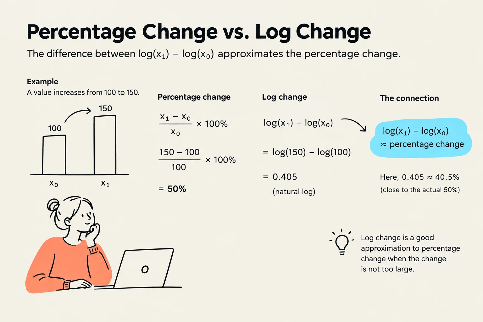
Finally, economists often use elasticity (ϵyx) to describe the sensitivity of one variable to another. It is defined as the percentage change in y per percentage change in x. Using the natural logarithm (log), we can approximate elasticity for small changes:
ϵyx≈Δlog(x)Δlog(y)
This illustration explains the relationship between percentage change and log change, demonstrating that log change is a good approximation for percentage change when the change is not too large.
Keep reading for free.
Create an account to finish this reading and make it part of your study routine.