This content explains the concept of price elasticity of demand, its calculation using the midpoint method, its categorization into elastic, inelastic, and unit elastic, and its relationship with total revenue and factors influencing it.
In economics, we understand through the law of demand that there is an inverse relationship between price and quantity demanded: when the price of a good rises, the quantity demanded typically falls. However, this law only tells us the direction of the change. It does not tell us the magnitude. If the price of an ambulance ride increases, will people stop using them entirely, or will they continue to pay the higher price because they have no choice? To answer this, economists use a concept called elasticity.
What is Price Elasticity of Demand?
Price elasticity of demand measures the responsiveness of the quantity demanded to a change in price. Essentially, it quantifies how much consumers "stretch" or "shrink" their purchasing behavior when a price tag changes.
To calculate this, we look at the relationship between two specific values: the percentage change in quantity demanded and the percentage change in price. The formula is expressed as:
Price elasticity of demand=% change in price% change in quantity demanded
Because price and quantity move in opposite directions, the result of this calculation is usually negative. However, economists typically drop the minus sign and use the absolute value (∣Ed∣) for easier interpretation.
Exam Tip: Elasticity is not the same as the slope of a demand curve. However, if two linear demand curves pass through the same point, the flatter curve is the more elastic one.
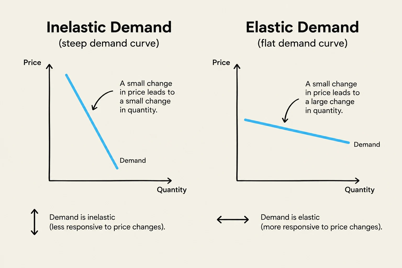
This image illustrates the concepts of inelastic and elastic demand using graphs. Inelastic demand is shown with a steep curve, indicating that price changes have a small effect on quantity demanded. Elastic demand is depicted with a flat curve, showing that price changes have a large effect on quantity demanded.
Categorizing Demand: Elastic, Inelastic, and Unit Elastic
Once we have calculated the elasticity coefficient, we can categorize the demand into several distinct types:
1. Elastic Demand (∣Ed∣>1)
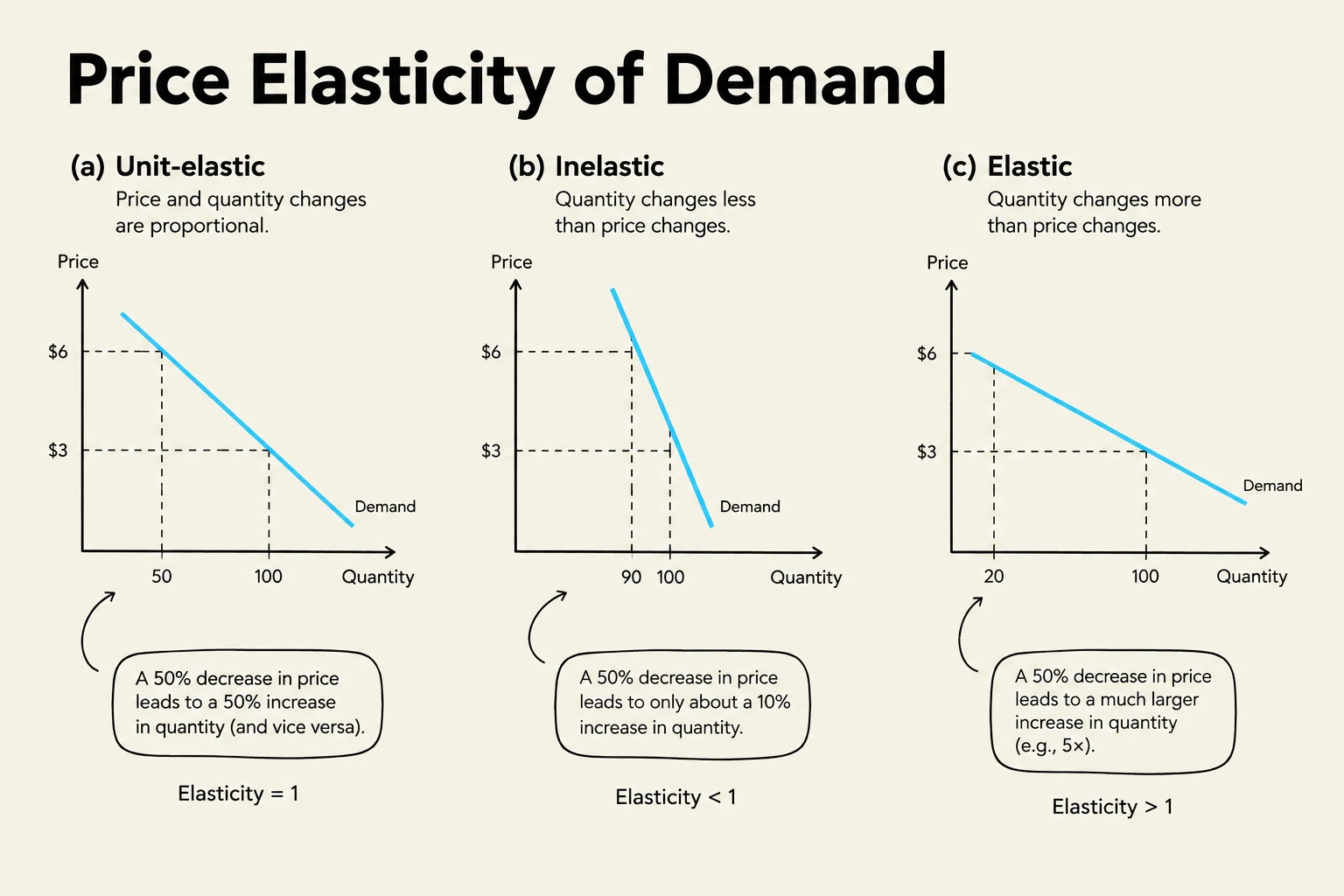
Demand is considered elastic when a change in price leads to a disproportionately large change in quantity demanded. In other words, consumers are very responsive to price changes. If a small price increase causes a "big decrease" in quantity, the demand is elastic.
2. Inelastic Demand (∣Ed∣<1)
Demand is inelastic when a change in price results in a relatively small change in quantity demanded. Consumers are not very responsive to price fluctuations. For example, if a price increase causes only a "small decrease" in quantity, the demand is inelastic.
3. Unit Elastic Demand (∣Ed∣=1)
Demand is unit elastic when the percentage change in quantity demanded is exactly equal to the percentage change in price. In this scenario, the two effects balance each other out perfectly.
4. Perfectly Inelastic Demand (Ed=0)
In the extreme case of perfectly inelastic demand, the quantity demanded does not change at all, regardless of how much the price rises or falls. An example might be a life-saving medication where the quantity needed remains constant regardless of cost.
5. Perfectly Elastic Demand (Ed=∞)
The opposite extreme is perfectly elastic demand. Here, at a specific price, consumers will buy any quantity, but if the price rises even slightly above that level, the quantity demanded drops to zero.
The image illustrates the concept of price elasticity of demand with three graphs: unit-elastic, inelastic, and elastic demand. Each graph shows the relationship between price and quantity demanded, with explanations of how changes in price affect quantity demanded in each scenario.
Measuring Elasticity: The Midpoint Method
A common problem when calculating percentage changes is that the result depends on whether you are calculating a price increase or a price decrease. To solve this, economists use the midpoint formula. Instead of using the initial value as the base, the midpoint method uses the average of the starting and final values.
The formula for the percentage change of a variable X using the midpoint method is:
% change in X=(2Xfinal+Xinitial)Xfinal−Xinitial×100
This ensures that the elasticity remains the same whether the price is moving up or down between two points.
Elasticity and Total Revenue
For sellers, understanding elasticity is vital for planning because it dictates how price changes will affect Total Revenue (TR), where TR=Price×Quantity.
Inelastic Demand: The "price effect" dominates the "quantity effect." If you raise the price, the slight drop in quantity sold is outweighed by the higher price per unit, so total revenue rises.
Elastic Demand: The "quantity effect" dominates. A price increase causes such a significant drop in quantity that total revenue falls.
Unit Elastic Demand: The price effect and quantity effect exactly balance each other, meaning total revenue does not change.
What Determines Elasticity?
Several factors influence how sensitive consumers are to price changes:
Availability of Substitutes: This is a critical factor. If many close substitutes are available, demand is elastic because consumers can easily switch brands.
Necessity vs. Luxury: Necessities tend to have inelastic demand, while luxuries are more price-sensitive and thus elastic.
Share of Income: Goods that take up a large portion of a consumer's budget tend to be more elastic than "cheap" goods.
Time Elapsed: Demand becomes more elastic over time as consumers find ways to adjust their behavior or find substitutes.
Keep reading for free.
Create an account to finish this reading and make it part of your study routine.