Data Classification and Summarizing Categorical Variables

Numerical Variables

Numerical variables represent quantities. Unlike categorical variables, a numerical observation can take on any integer or non-integer value within a given range. These are often called "measured" variables because they represent a scale of measurement.

Numerical variables are classified into two types:

1. Discrete Variables: These variables take on distinct, separate values, usually integers. You cannot have half a student in a class or $2.5$ shares owned; these counts jump from one whole number to the next.
2. Continuous Variables: These variables can assume any value within a certain range, including decimals and fractions. Common examples include weight (kg), income ($), and age (years).

Student Tip: The "Average" Trap A common mistake is attempting to calculate the mean (average) of a categorical variable. For example, if you assign "1" to "Cat" and "2" to "Dog," calculating an average of $1.5$ is mathematically possible but logically meaningless. You cannot be "halfway between a cat and a dog." Always check your variable type before choosing a summary statistic!

Summarising One Categorical Variable

Once you have identified a variable as categorical, you need a way to describe it to others. Because you cannot calculate a mean or median for categories, you must rely on counts, proportions, and the mode.

Frequency Tables

The most fundamental way to summarize a single categorical variable is to construct a frequency table. A professional frequency table should include:

• The name of the variable being studied.
• The name of each distinct category.
• The count (the number of observations in each category).
• The proportion or percentage of observations in each category.
• The total sample size, denoted as $n$.

To calculate these values:

• Proportion: $\frac{\text{Count of Category}}{\text{Total Sample Size } (n)}$
• Percentage: $\text{Proportion} \times 100$

The Mode

The mode is the simplest measure of central tendency for categorical data. It is defined as the most common observation that appears in your dataset.

If your data consists of words: $\text{(Cat, Dog, Snake, Cat, Dog, Dog, Snake)}$ The category "Dog" appears three times, while "Cat" and "Snake" appear only twice. Therefore, "Dog" is the mode.

If your data is coded numerically (where numbers represent categories): $\text{(1, 2, 3, 1, 2, 2, 3)}$ Here, if $1 = \text{Cat}$, $2 = \text{Dog}$, and $3 = \text{Snake}$, the number $2$ is the mode because it occurs most frequently.

Graphical Representations

Visualizing categorical data allows for quick identification of patterns and distributions. Two primary methods are used:

Pie Charts

A pie chart represents the distribution of categories as slices of a circle, where the size of each slice corresponds to the percentage of the total. This is particularly useful for showing how a whole is divided into various parts.

Bar Charts

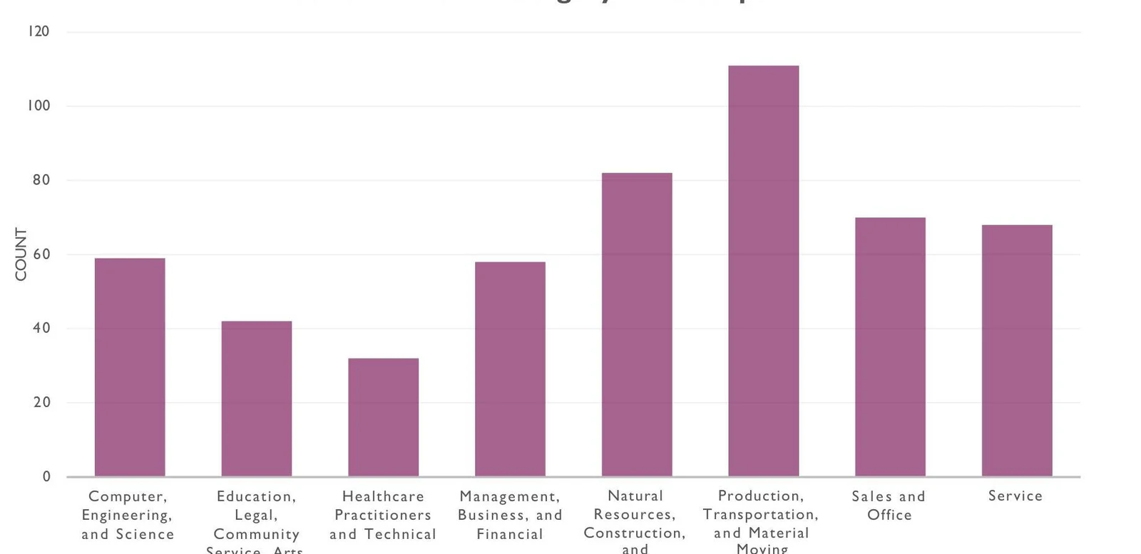
A bar chart uses rectangular bars to represent the counts (or frequencies) of each category. The height of each bar corresponds to the frequency of that specific category, making it easy to compare the relative sizes of different groups at a glance.

Exam Tip: Pie Chart vs. Bar Chart Use a pie chart when you want to emphasize how much each category contributes to a "whole" (e.g., market share). Use a bar chart when you want to compare the absolute sizes of different categories or when you have many categories that would make a pie chart look cluttered and unreadable.

Summary Table of Variable Types

By mastering these classifications and summary techniques, you ensure that your statistical analysis is both mathematically sound and communicable to your audience.