Controlling for Confounding Variables in Regression

1. t-value: This indicates how much evidence there is that a regression coefficient is different from zero. A large t-value suggests strong evidence of an effect, while a t-value close to zero suggests little to no effect.
2. p-value: This tells you the statistical significance of the coefficient. Typically, if $p < .05$, the relationship is considered statistically significant.
3. Confidence Interval: This provides a range of values within which the true population coefficient is likely to fall. If the interval does not include zero, the effect is considered statistically significant.
4. Standardised Regression Coefficients ($\beta$): These are used to compare the relative strength of different predictors within the same model, as they are measured in standard deviation units.

Understanding Confounding

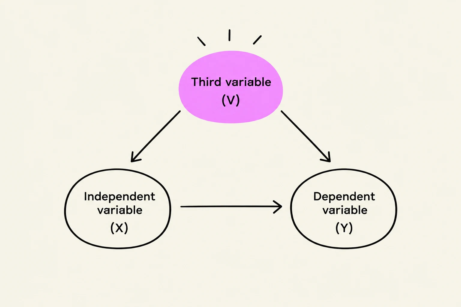
A confounder is a variable that is associated with both the independent variable and the dependent variable. If you do not include a confounder in your model, the relationship you observe between $X$ and $Y$ might be "spurious"—meaning it isn't a direct relationship, but rather a byproduct of the confounder's influence.

Example Scenario: Imagine we study the effect of News Exposure ($X$) on Political Participation ($Y$). We might find a strong positive relationship. However, Political Interest ($Z$) might be a confounder: people with high political interest tend to watch more news and tend to participate more in politics.

Controlling for Confounders: Four Possible Outcomes

When you run a second regression model that includes the confounder (e.g., $Y$ predicted by $X$ and $Z$), the regression coefficient for $X$ will change. By comparing the first model (without $Z$) to the second model (with $Z$), you can identify one of four outcomes:

1. The effect disappears: The coefficient for $X$ drops toward zero and becomes non-significant ($p > .05$). This means the original relationship was entirely explained by the confounder (a spurious relationship).
2. The effect becomes smaller: The coefficient for $X$ decreases but remains significant. This is called partial confounding, meaning $Z$ explains part of the relationship, but $X$ still has its own unique effect.
3. The effect remains unchanged: The coefficient for $X$ stays roughly the same. This suggests the confounder does not explain the relationship between $X$ and $Y$.
4. The effect becomes stronger or changes direction: This is known as suppression or negative confounding. The confounder was actually "masking" the true relationship, making it appear weaker or even opposite in direction than it actually is.

Worked Example: Interpreting the Model

Let's apply this to our news exposure example. Suppose we run a model where Political Participation is predicted by News Exposure and Political Interest.

The Regression Equation:

$$\begin{aligned} \text{Political Participation} &= .55 + .34 \cdot \text{News Exposure} + .62 \cdot \text{Political Interest} \end{aligned}$$

How to interpret these values:

• Intercept (.55): The predicted score for political participation is .55 when both news exposure and political interest are zero.
• Slope for News Exposure (.34): If news exposure increases by 1 unit, political participation is predicted to increase by .34 units, while controlling for political interest.
• Slope for Political Interest (.62): If political interest increases by 1 unit, political participation is predicted to increase by .62 units, while controlling for news exposure.

Exam Tip: Calculating Predicted Scores If an exam asks you to predict the score for someone with a News Exposure of 7 and Political Interest of 7, plug the numbers directly into the equation:

$$\begin{aligned} Y &= .55 + (.34 \cdot 7) + (.62 \cdot 7) \\ Y &= .55 + 2.38 + 4.34 \\ Y &= 7.27 \end{aligned}$$

Always use the maximum number of decimal places provided in your output to ensure accuracy.

Final Check: Homoscedasticity

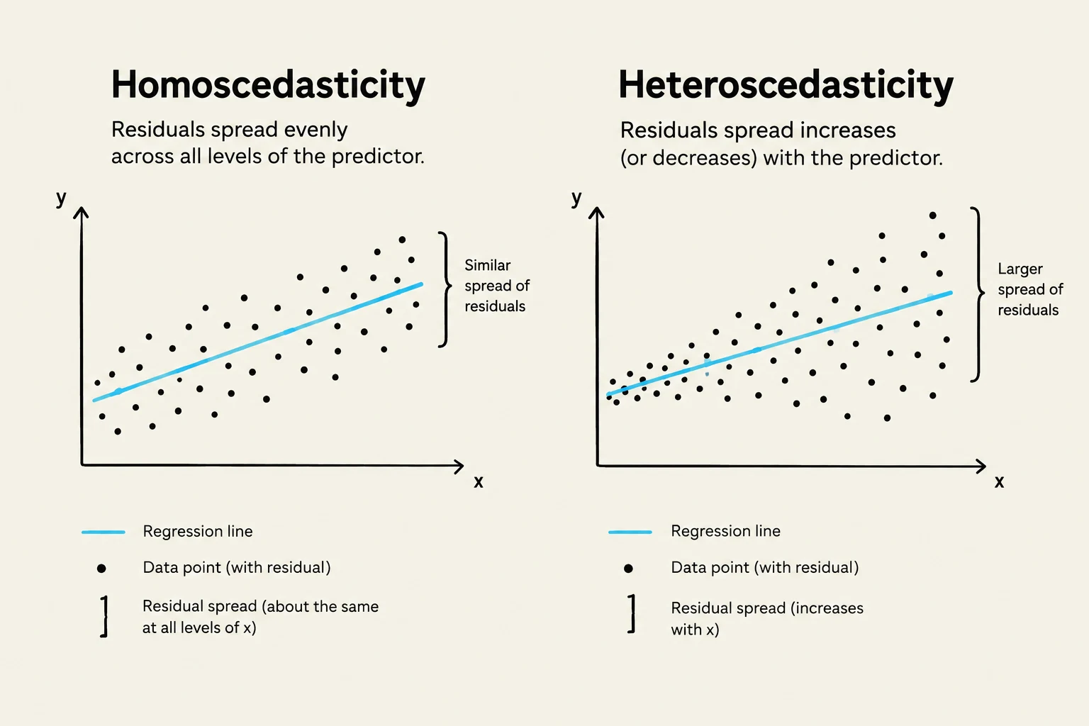
After running your regression, you must ensure the model's assumptions are met. One critical assumption is homoscedasticity. This means that the "residuals" (the errors or the differences between predicted and actual values) should be approximately equally spread around the regression line.

If the spread of errors increases or decreases as your predictor changes (creating a "funnel" shape), you have heteroscedasticity, and your model's reliability may be compromised.