Explores consumer behavior in microeconomics, covering total and marginal utility, the law of diminishing marginal utility, ordinal utility, indifference curves, marginal rate of substitution, budget constraints, and consumer equilibrium.
In microeconomics, the study of consumer behavior seeks to explain how individuals make choices to satisfy their needs and wants. Acting as rational agents, consumers aim to maximize their economic utility—the satisfaction derived from goods and services—while operating under the reality of limited resources. This article explores the transition from cardinal utility to the modern ordinal approach, ultimately determining how a consumer reaches an optimal equilibrium.
The Foundations of Utility: Total and Marginal
To understand how consumers make decisions, we must first define how they measure satisfaction.
Total Utility (U) represents the overall satisfaction an individual obtains from consuming a specific quantity of a good. It is expressed as a function of the quantity consumed:
U=f(X)
Marginal Utility (Um) measures the change in total utility resulting from a small change in consumption. For goods that are perfectly divisible (meaning they can be consumed in infinitely small increments), marginal utility is mathematically defined as the derivative of the total utility function with respect to the quantity X:
Um=∂X∂U
The Law of Diminishing Marginal Utility
A fundamental principle in consumer theory is the Law of Diminishing Marginal Utility. This principle suggests that as a person consumes more and more of a specific good, the additional satisfaction gained from each subsequent unit decreases.
Eventually, consumption reaches a saturation point (or satiety point), where marginal utility becomes zero. Beyond this point, consuming more of the good actually leads to a decrease in total utility, as the marginal utility becomes negative.
This image displays two graphs. The top graph shows a curve labeled U=f(x) with U on the y-axis and X on the x-axis. The curve starts at the origin and rises to a peak labeled S before descending. The bottom graph shows a curve labeled Um=dU/dX, with Um on the y-axis and X on the x-axis. This curve starts high on the y-axis and decreases as X increases, crossing the x-axis.Figure 3.1: The relationship between total utility and marginal utility.
The Ordinal Utility Approach
While early economists used "cardinal utility" (assigning absolute numbers to satisfaction), modern theory utilizes an ordinal approach. This approach assumes that consumers can rank their preferences (e.g., "I prefer bundle A to bundle B") without needing to assign a specific numerical value to the satisfaction level.
Indifference Curves
The primary tool of ordinal theory is the indifference curve (or iso-utility curve). An indifference curve represents all possible combinations of two goods (X and Y) that provide the consumer with the exact same level of total utility.
Key properties of indifference curves include:
Downward Sloping: To maintain the same utility, if a consumer consumes more of good X, they must consume less of good Y.
Convex to the Origin: The curves are bowed toward the axes, reflecting the consumer's willingness to trade goods at varying rates.
Non-intersecting: Two indifference curves can never cross, as this would violate the principle of logical preference.
Figure 3.3: Indifference curves representing different levels of utility.
Marginal Rate of Substitution (RMS)
The slope of the indifference curve at any given point is known as the Marginal Rate of Substitution (RMS). It measures the rate at which a consumer is willing to substitute good Y for good X to maintain the same level of utility. Mathematically, it is expressed as:
RMS=−∂X∂Y
Exam Tip: Remember that the RMS is the "slope at a point" on the indifference curve. Because indifference curves are convex, the RMS decreases as you move down the curve from left to right.
Budget Constraints and Consumer Equilibrium
A consumer cannot simply choose any point on an indifference curve; they are limited by their available income and the prices of goods.
The Budget Constraint
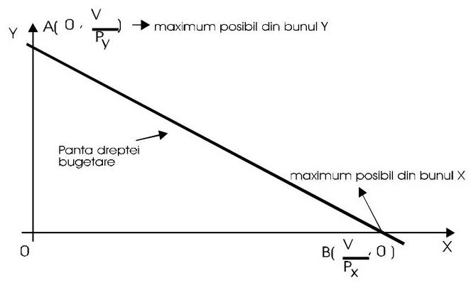
The budget constraint represents the limit on consumption imposed by the consumer's income (V) and the prices of the goods (Px and Py). The equation for the budget line is:
V=Px⋅X+Py⋅Y
The slope of the budget line is −PyPx, which represents the market rate at which the two goods can be exchanged.
A budget line graph showing the maximum possible combinations of two goods (X and Y) that can be purchased given a budget (V) and prices (Px and Py). The slope of the budget line represents the trade-off between the two goods.Figure 3.4: The construction of a budget line.
Optimal Choice (Consumer Equilibrium)
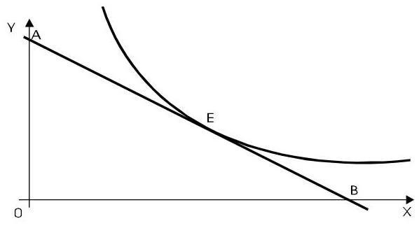
The optimal choice, or consumer equilibrium, occurs when the consumer reaches the highest possible indifference curve that is still within their budget constraint. Graphically, this is the point where the budget line is tangent to the indifference curve.
At this equilibrium point, the rate at which the consumer is willing to trade goods (RMS) equals the rate at which the market allows them to trade goods (PyPx). This can be expressed in two equivalent ways:
RMS=PyPxPxUmX=PyUmY
A graph showing a curve tangent to a line at point E.Figure 3.5: The point of tangency (E) represents the optimal consumer choice.
Effects of Price and Income Variations
Changes in the economic environment shift the equilibrium point by altering the budget constraint.
Price Variation Effects
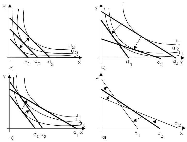
When the price of one good changes (while income and the other price remain constant), the budget line rotates around the intercept of the unaffected good.
If Px decreases, the budget line rotates outward along the X-axis, increasing the consumer's real income (purchasing power) and allowing them to reach a higher indifference curve.
If Px increases, the budget line rotates inward, reducing purchasing power and utility.
These diagrams illustrate indifference curves and budget lines in economics, showing consumer choice and utility maximization under different scenarios.Figure 3.6: Visualizing the shift in equilibrium due to price changes.
Income Variation Effects
When nominal income (V) changes but prices remain constant, the budget line undergoes a parallel shift.
Increase in Income: The budget line shifts outward (to the right), allowing the consumer to reach higher indifference curves and higher levels of utility.
Decrease in Income: The budget line shifts inward (to the left), forcing the consumer to a lower indifference curve and a lower standard of living.
Worked Example: Finding the Optimal Bundle
Problem: A consumer has a utility function U=X(Y−2). The income is V=50, the price of X is Px=10, and the price of Y is Py=5. Find the optimal consumption bundle.
Solve the System of Equations:
Adding the two equations:
(10X−5Y+10)+(10X+5Y−50)=020X−40=0⟹X=2
Substitute X=2 into the budget equation:
10(2)+5Y=50⟹20+5Y=50⟹5Y=30⟹Y=6
Result: The optimal bundle is 2 units of X and 6 units of Y.
Keep reading for free.
Create an account to finish this reading and make it part of your study routine.