Learn how to calculate recombination frequency to understand gene linkage and genetic mapping. This guide covers independent assortment, crossing over, testcrosses, and the chi-square test.
In classical Mendelian genetics, we often assume that genes for different traits assort independently. This means the inheritance of one trait does not influence the inheritance of another. However, genes are physical entities located on chromosomes. When two genes are located close to one another on the same chromosome, they are said to be "linked". Because they are physically tied together, they do not follow the standard rules of independent assortment, but instead tend to be inherited together.
By studying the patterns of inheritance in offspring, geneticists can determine whether genes are linked and even estimate the physical distance between them on a chromosome. This process is known as genetic mapping.
Independent Assortment vs. Linkage
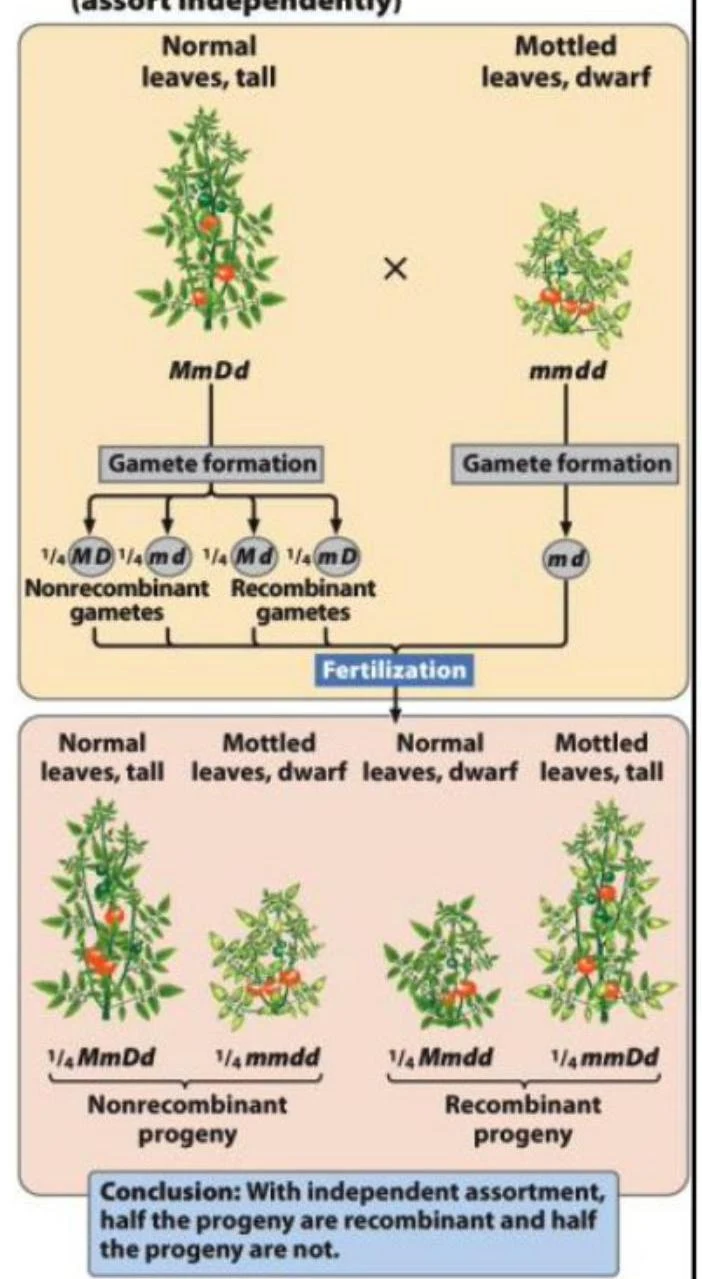
To understand linkage, we must first look at the baseline: independent assortment. According to Mendel's principles, alleles at different loci separate independently during meiosis. In a typical dihybrid testcross (crossing a heterozygote with a homozygous recessive individual), we expect to see four different phenotypes in equal proportions (a 1:1:1:1 ratio).
This diagram illustrates the principles of independent assortment in genetics, showing how alleles for different traits segregate independently during gamete formation and fertilization, leading to recombinant and nonrecombinant progeny.
When genes are linked, this 1:1:1:1 ratio is disrupted. Instead of seeing equal numbers of all four types, we see a disproportionately high number of "parental" types and a much lower number of "new" combinations.
Complete Linkage
In a theoretical scenario called complete linkage, no crossing over occurs between the two loci. In this case, the genes are so tightly bound that they always move together during meiosis. As a result, 100% of the progeny will exhibit the same combinations of traits seen in the parents (the nonrecombinant phenotypes).
Crossing Over and Recombination
In reality, most linkage is not complete. During Prophase I of meiosis, homologous chromosomes pair up and exchange segments of DNA in a process called crossing over.
Diagram illustrating the stages of meiosis I and meiosis II, including crossing over and the formation of gametes.
This exchange creates new combinations of alleles that were not present in the parents. These new combinations are found in the recombinant progeny. The offspring that maintain the original parental allele combinations are called nonrecombinant progeny.
The Testcross and Allele Configuration
To study these patterns effectively, scientists often use a testcross. A testcross involves crossing an individual with an unknown or heterozygous genotype with an individual that is homozygous recessive for all traits being studied. This is useful because the homozygous recessive parent can only contribute recessive alleles, meaning the phenotype of the offspring directly reveals the alleles present in the gametes of the heterozygous parent.
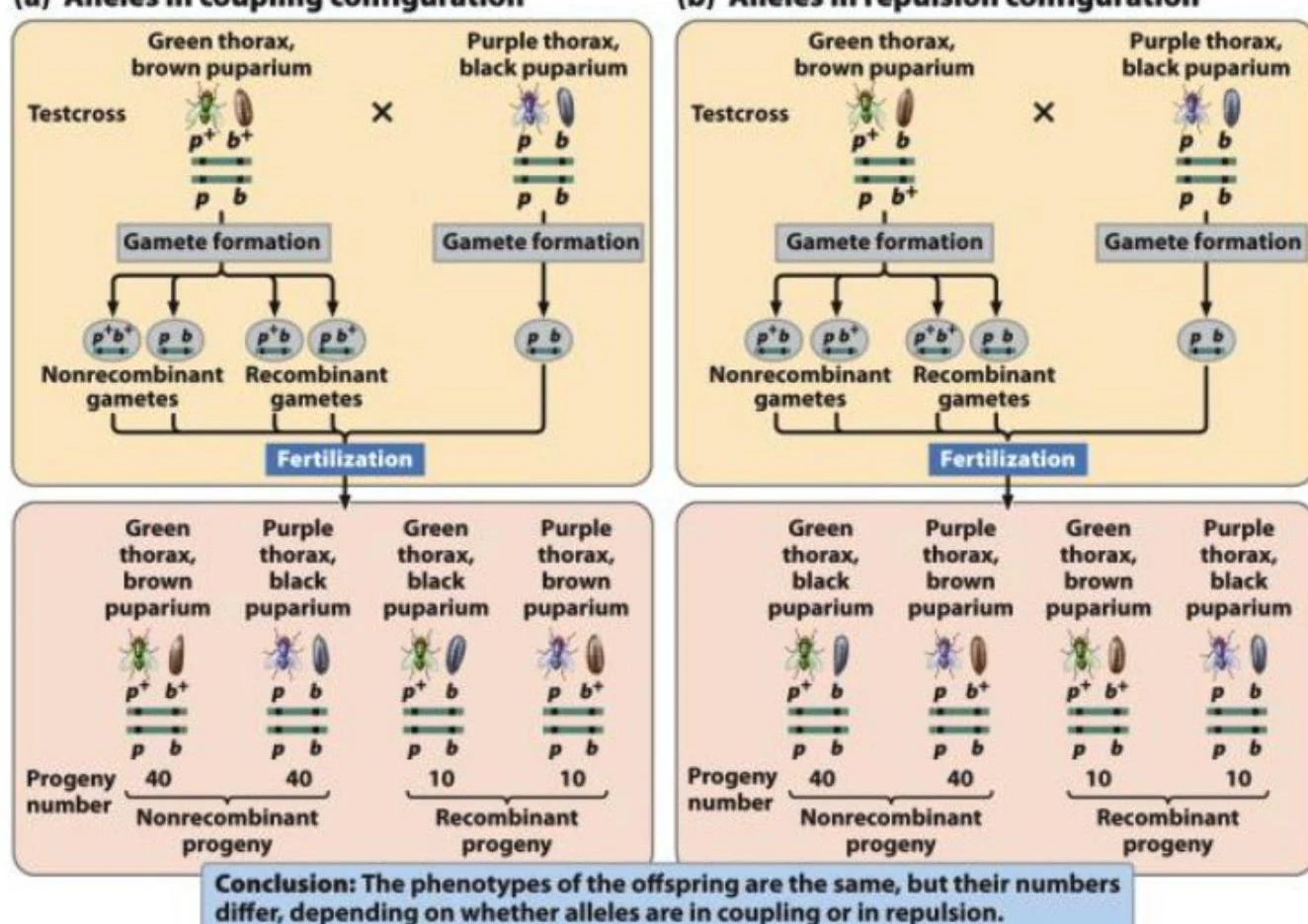
When analyzing these crosses, the arrangement of alleles on the chromosomes is critical. There are two main configurations:
Coupling (Cis) configuration: The dominant (or wild-type) alleles for both genes are on one chromosome, and the recessive alleles are on the other.
Repulsion (Trans) configuration: Each chromosome carries one dominant allele and one recessive allele.
This diagram illustrates genetic linkage and recombination in fruit flies. It shows two scenarios: alleles in coupling configuration and alleles in repulsion configuration. The testcross results in different proportions of nonrecombinant and recombinant progeny depending on the initial arrangement of alleles, demonstrating how linkage affects inheritance patterns.
Calculating Recombination Frequency
The recombination frequency is the percentage of recombinant progeny produced in a cross. This value is a direct reflection of how often crossing over occurs between two specific loci. Because crossing over is more likely to happen if two genes are far apart, the recombination frequency serves as a measure of the physical distance between genes.
To calculate the frequency, use the following formula:
recombination frequency=total number of progenynumber of recombinant progeny×100%
Worked Example
Imagine a testcross of tomato plants where you observe the following progeny counts:
Normal leaves, tall (Nonrecombinant): 55
Mottled leaves, dwarf (Nonrecombinant): 53
Normal leaves, dwarf (Recombinant): 8
Mottled leaves, tall (Recombinant): 7
Step 1: Identify the recombinant progeny.
The recombinant progeny are the ones with the "new" combinations (8 and 7).
Step 2: Calculate the total number of progeny.Total=55+53+8+7=123
Step 3: Apply the formula.recombination frequency=1238+7×100%recombination frequency=12315×100%≈12.2%
Exam Tip: Always remember that recombinant progeny are the least numerous groups in a linkage cross. If you are looking at a data set and the "new" combinations have much lower counts than the "parental" combinations, you are looking at linked genes.
Predicting Outcomes and Genetic Mapping
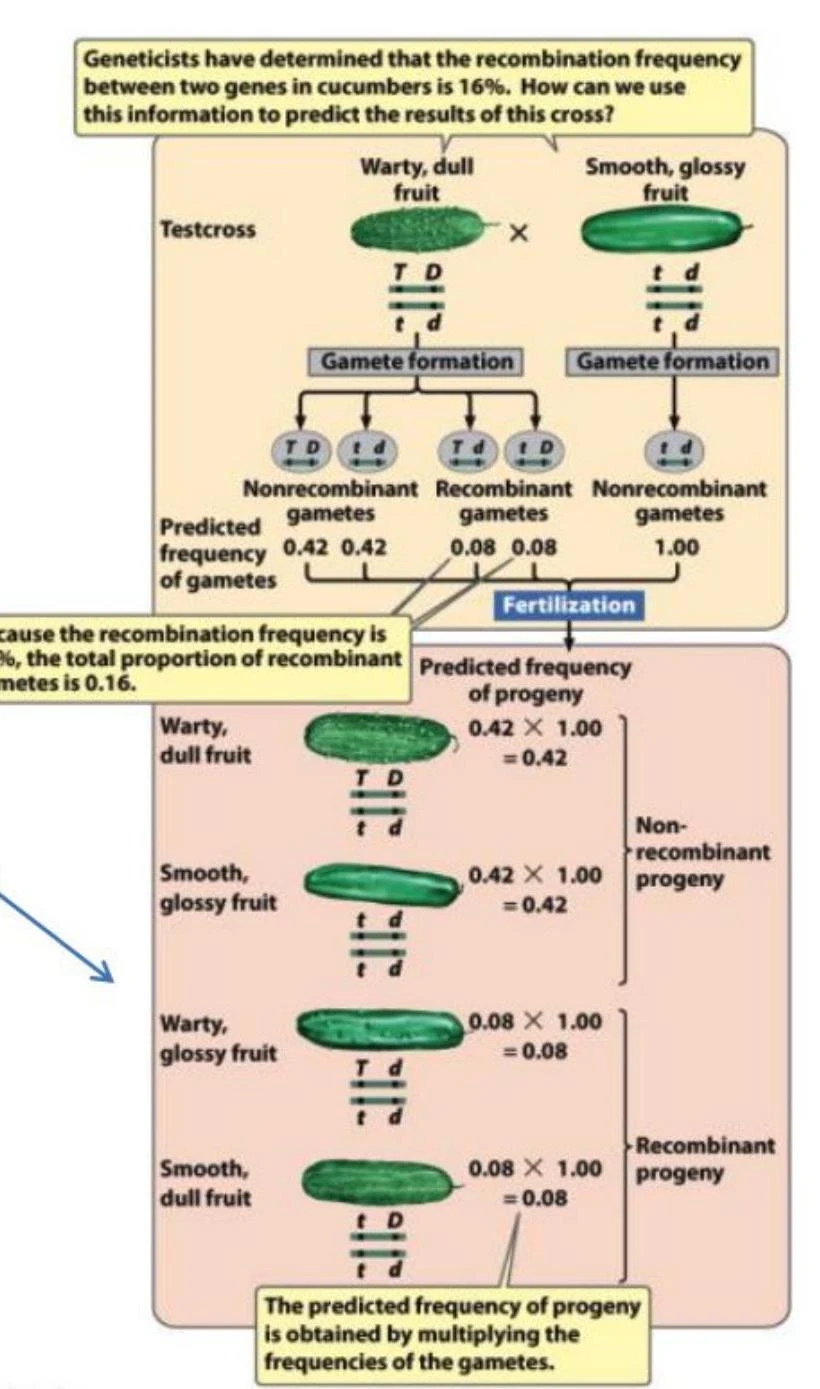
Once you know the recombination frequency, you can use the multiplication rule to predict the probability of specific offspring genotypes in future crosses. In a testcross, the probability of the recessive parent contributing a recessive allele is always 1, so you only need to calculate the probability of the gametes produced by the heterozygous parent.
This diagram illustrates how recombination frequency between two genes in cucumbers can be used to predict the results of a genetic cross, showing the formation of gametes and the predicted frequency of progeny.
This ability to predict proportions and the relationship between recombination and physical distance allows scientists to perform genetic mapping. By calculating these frequencies for multiple genes, we can determine the relative order and distance of genes along a chromosome, creating a map of the genome.
Statistical Validation: The Chi-Square Test
How do we know if the deviation from the expected 1:1:1:1 ratio is actually due to linkage, or just random chance? To distinguish between these, we use a Chi-square (χ2) test of independence.
Unlike a standard goodness-of-fit test, the test of independence uses a contingency table to see if the segregation of alleles at one locus is independent of the segregation at another.
Create a contingency table: Organize observed counts by the two different traits.
Calculate expected values: For each cell, multiply the row total by the column total and divide by the grand total.
Expected=Grand TotalRow Total×Column Total
Calculate χ2:
χ2=∑expected(observed−expected)2
Determine Significance: Compare your χ2 value to a critical value from a distribution table using the appropriate degrees of freedom (df=(rows−1)×(cols−1)).
If the calculated χ2 is higher than the critical value (resulting in a P<0.05), we reject the hypothesis of independent assortment and conclude that the genes are linked.
Keep reading for free.
Create an account to finish this reading and make it part of your study routine.