An introduction to the fundamental concepts of statistics, including population, samples, variables, and the classification of data. It covers descriptive statistics, measures of central tendency (mean, median, mode), and measures of dispersion (range, variance, standard deviation).
Statistics is a powerful selection of mathematical tools and techniques used to summarize, interpret, and analyze data, particularly when dealing with uncertain systems or environments. Because many real-world systems are too large, complex, or fast-changing to observe in their entirety, we rely on the processes of sampling and estimation to understand them.
Population, Samples, and Variables
Before performing calculations, we must define the scope of our study. A population represents the entire set of units of interest—for example, every high school student currently enrolled in a specific school. Because observing an entire population is often impossible, we collect a sample, which is a subset of that population.
The relationship between these groups is defined by the types of values we calculate:
Parameters: Numerical descriptors calculated using the entire population.
Statistics: Numerical descriptors calculated from a sample, used to estimate the population parameters.
Within these groups, we look at variables, which are specific characteristics of a system. A single recorded value from a population or sample is known as an observation.
Classifying Variable Types
Not all data is created equal. Variables are generally classified into two main categories: categorical and numerical.
Categorical Variables
These describe qualities or groups rather than quantities:
Nominal: Unordered categories where the sequence does not matter (e.g., color or region).
Ordinal: Ordered categories where the sequence matters, but the mathematical distance between them is not quantifiable (e.g., education level or satisfaction ratings).
Binary (Dichotomous): A special case of categorical data containing only two options, such as Yes/No or Male/Female.
Numerical Variables
These describe quantities and are further divided by how they are measured:
Count/Discrete: Integers representing counts of items (e.g., the number of children in a household).
Continuous: Real numbers that arise from measurements (e.g., height, weight, or temperature).
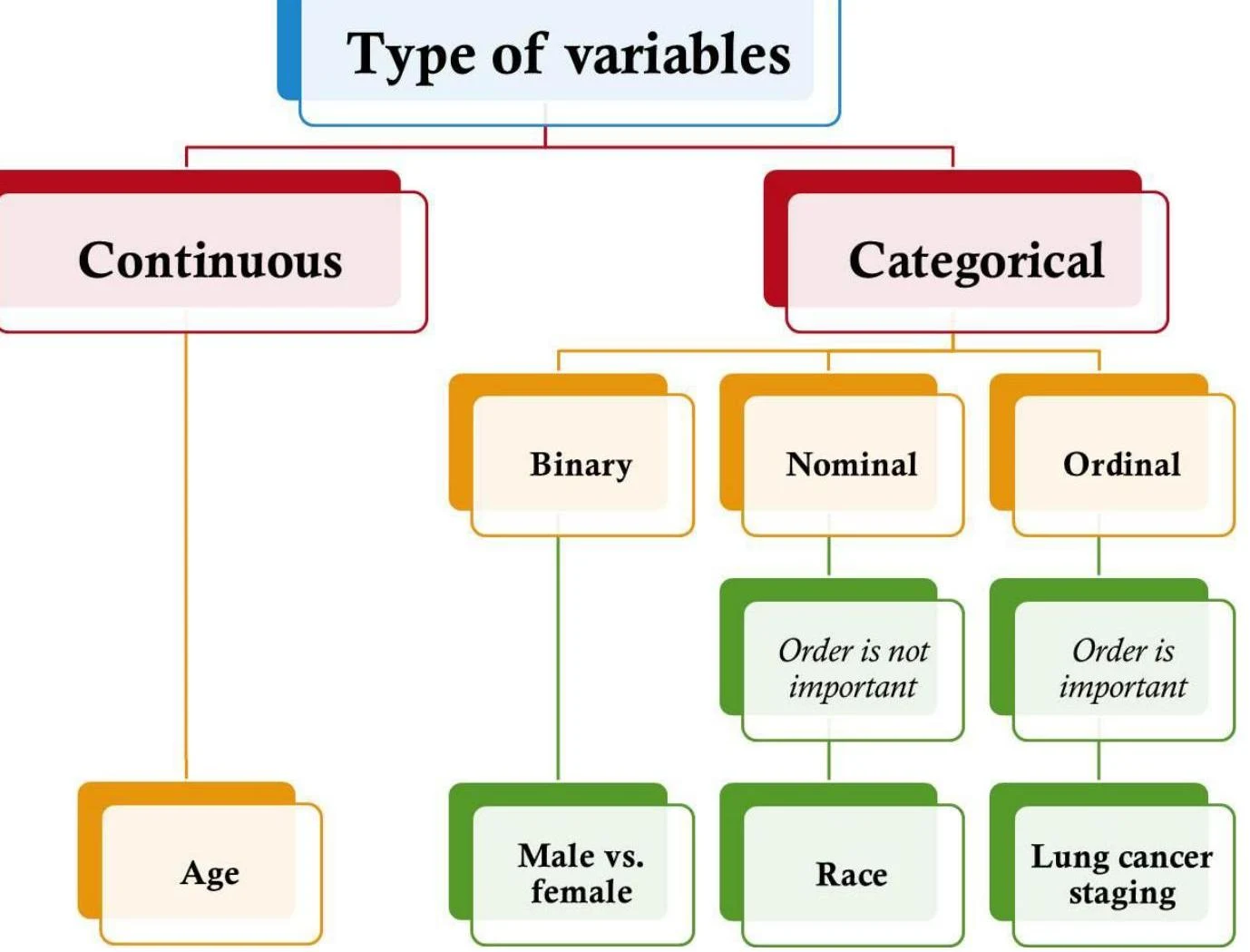
This diagram illustrates the classification of variables into continuous and categorical types, with further subdivisions for categorical variables like binary, nominal, and ordinal, along with examples.
Descriptive Statistics: Univariate vs. Multivariate
Descriptive statistics serve as the foundation for all quantitative analysis. They summarize data to present key characteristics such as the center, shape, and variability.
Univariate Statistics: These describe the distribution of a single variable by looking at its location, dispersion, and shape.
Multivariate Statistics: These describe the relationships between pairs of variables, using tools like correlations, covariance, and scatterplots.
Measures of Location (Central Tendency)
Measures of location help us identify the "center" or the "expected" value of a data series.
The Mean
The arithmetic mean is the most common measure of central tendency. It is calculated by adding all values and dividing by the total number of observations.
For a population of N values:
μ=N∑i=1Nxi
For a sample of size n:
xˉ=n∑i=1nxi
The Median
The median is the midpoint of a data series that separates the observations into two equal halves. To find it, you must first order the data.
Note on Calculation: The formula for the median position is (2n+1).
If n is odd, the median is the middle value.
If n is even, the median is the average of the two middle values.
The Mode
The mode is the most frequently observed value in a data series.
Position, Quartiles, and the 5-Number Summary
To understand where a specific value sits relative to the rest of the data, we use percentiles and quartiles.
Quartiles split an ordered dataset into four equal segments:
Q1 (First Quartile): 25% of observations are smaller than this value.
Q2 (Second Quartile): This is the Median (50% of observations are smaller).
Q3 (Third Quartile): 75% of observations are smaller than this value.
Worked Example: Finding Q1
Given the series: $11, 12, 13, 16, 16, 17, 18, 21, 22$ (n=9)
Find the position: Q1 position=0.25(n+1)=0.25(10)=2.5.
Since the position is 2.5, we take the midpoint between the 2nd value (12) and the 3rd value (13).
Q1=212+13=12.5.
By combining the Minimum, Q1, Median, Q3, and Maximum, we create a 5-number summary, which provides an immediate snapshot of the data's distribution.
Measures of Dispersion
While measures of location tell us where the center is, measures of dispersion tell us how "spread out" the data is.
Range: The difference between the maximum and minimum values.
Variance: A measure of the distance between each observation and the mean, squared.
Population Variance (σ2): σ2=N∑i=1N(xi−μ)2.
Sample Variance (s2): s2=n−1∑i=1n(xi−xˉ)2.
Standard Deviation (s or σ): The square root of the variance. This is often preferred because it uses the same units as the original data, making it easier to interpret.
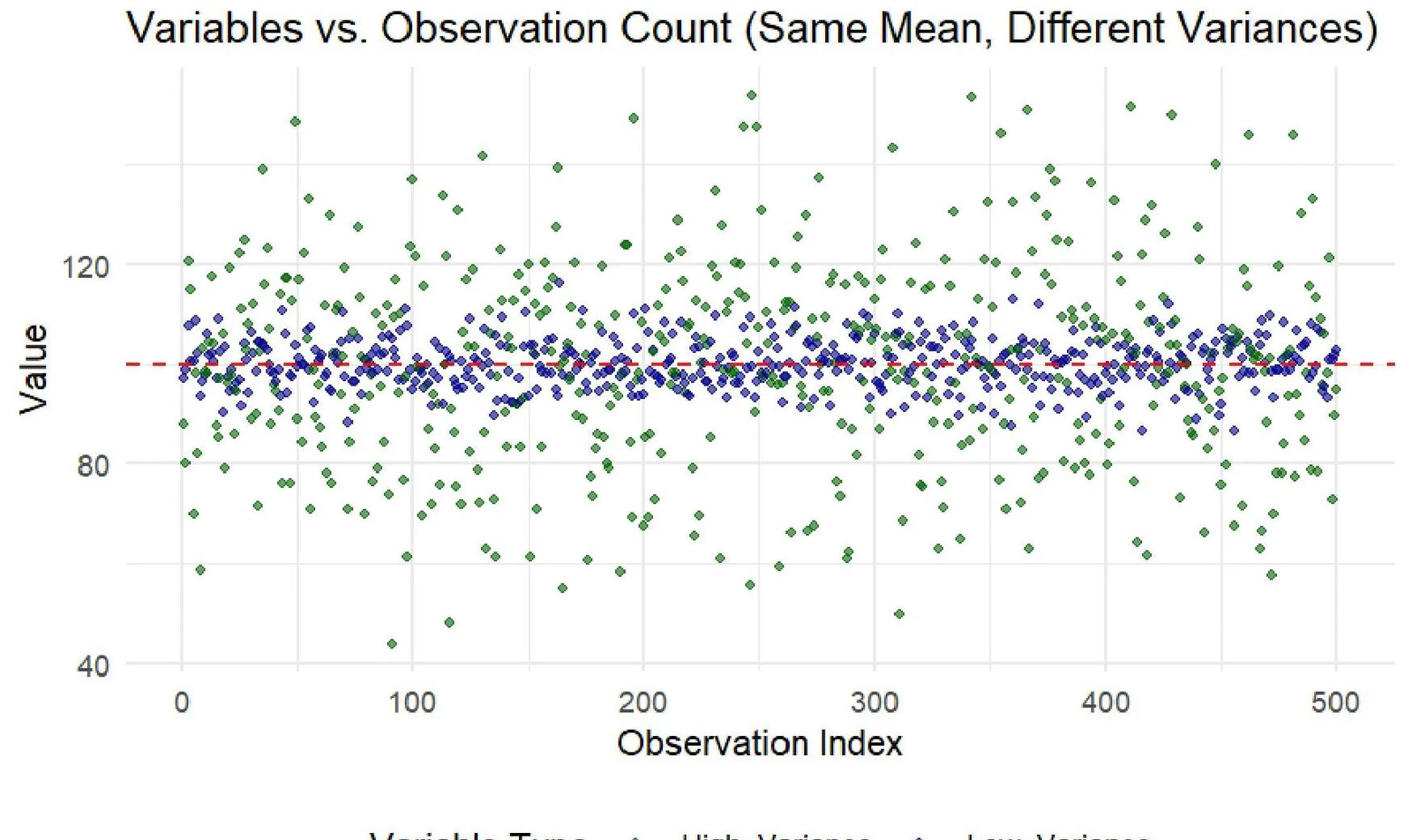
This scatter plot illustrates two variables with the same mean but different variances. The x-axis represents the observation index, and the y-axis represents the value. The dashed red line indicates the mean value. The blue dots represent data with low variance, while the green dots represent data with high variance.
The Coefficient of Variation (CoV)
To determine if a standard deviation is "high," we must compare it to the mean using the Coefficient of Variation.
CoV=Arithmetic MeanStandard Deviation
The CoV measures relative consistency. A high CoV (e.g., greater than 1) suggests the data is widely dispersed, meaning the average might not be a representative "typical" value for the majority of observations.
Keep reading for free.
Create an account to finish this reading and make it part of your study routine.