This guide explains how economists use graphs to visualize and understand economic relationships, covering direct, inverse, and independent relationships, the calculation of slope, and the distinction between movements along and shifts in curves.
Economists frequently use graphs because "a picture is worth a thousand words". While economic relationships can be expressed through verbal statements, tables, or equations, a graph provides the simplest way to visualize and understand how one variable affects another. By using a two-dimensional illustration, we can analyze the effects of a change in one variable on another within a coordinate system.
The Ceteris Paribus Assumption
Before diving into specific relationships, it is vital to understand how economic models are constructed. A two-variable graph isolates the relationship between two specific variables by holding all other potential influences constant. This is known as the ceteris paribus assumption.
For example, when graphing the relationship between annual income and personal computer expenditure, economists assume other factors—such as the price of computers or education levels—remain unchanged. If these "hidden" variables were allowed to change, the entire position of the graph might shift.
Types of Variable Relationships
Economic analysis typically focuses on how two variables move in relation to one another. Depending on their association, these relationships fall into three categories: direct, inverse, or independent.
1. Direct Relationship
A direct relationship (or positive association) occurs when two variables move in the same direction. If one variable increases, the other increases; if one decreases, the other decreases. Graphically, a direct relationship is expressed as an upward sloping curve or line.
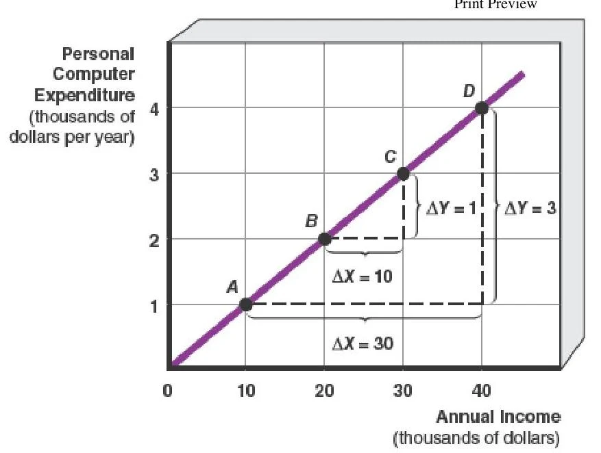
An example is the relationship between annual income and expenditure on personal computers. As annual income increases along the horizontal axis, the amount spent on a PC also increases on the vertical axis.
A graph illustrating the relationship between annual income and personal computer expenditure, showing a positive correlation. The graph includes points A, B, C, and D, with annotations indicating changes in X (Annual Income) and Y (Personal Computer Expenditure).
A table showing the relationship between personal computer expenditure and annual income, with data points labeled A, B, C, and D.
2. Inverse Relationship
An inverse relationship (or negative association) occurs when variables move in opposite directions. When one variable increases, the other decreases. This is expressed graphically as a downward sloping curve or line.
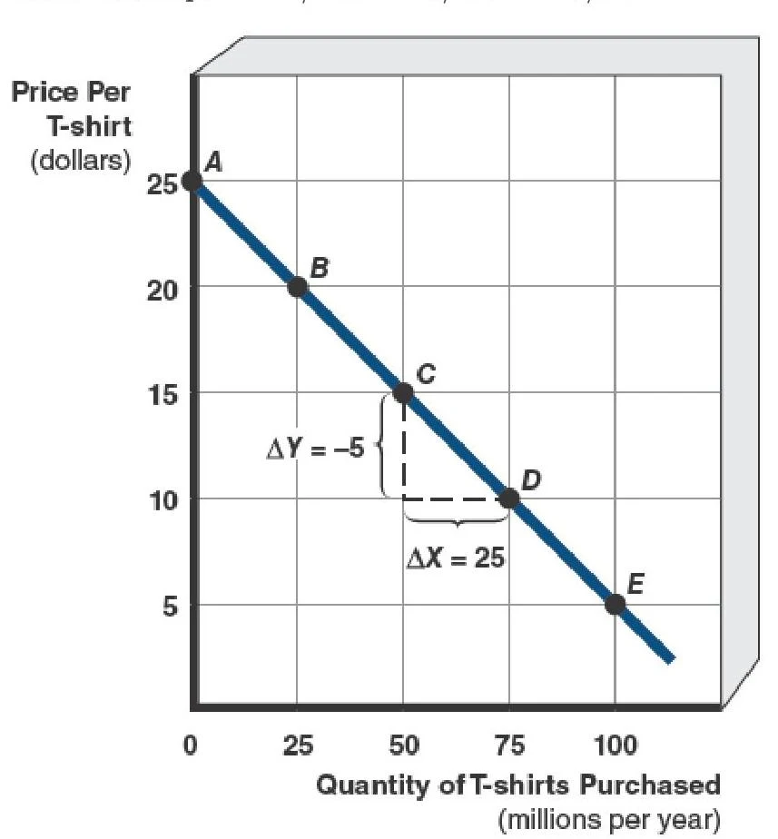
A classic example is the relationship between the price of T-shirts and the quantity consumers purchase. As the price of a T-shirt rises, the quantity purchased falls.
A graph illustrating the relationship between the price of t-shirts and the quantity purchased, showing a downward sloping demand curve with points labeled A through E and indicating changes in quantity and price.
3. Independent Relationship
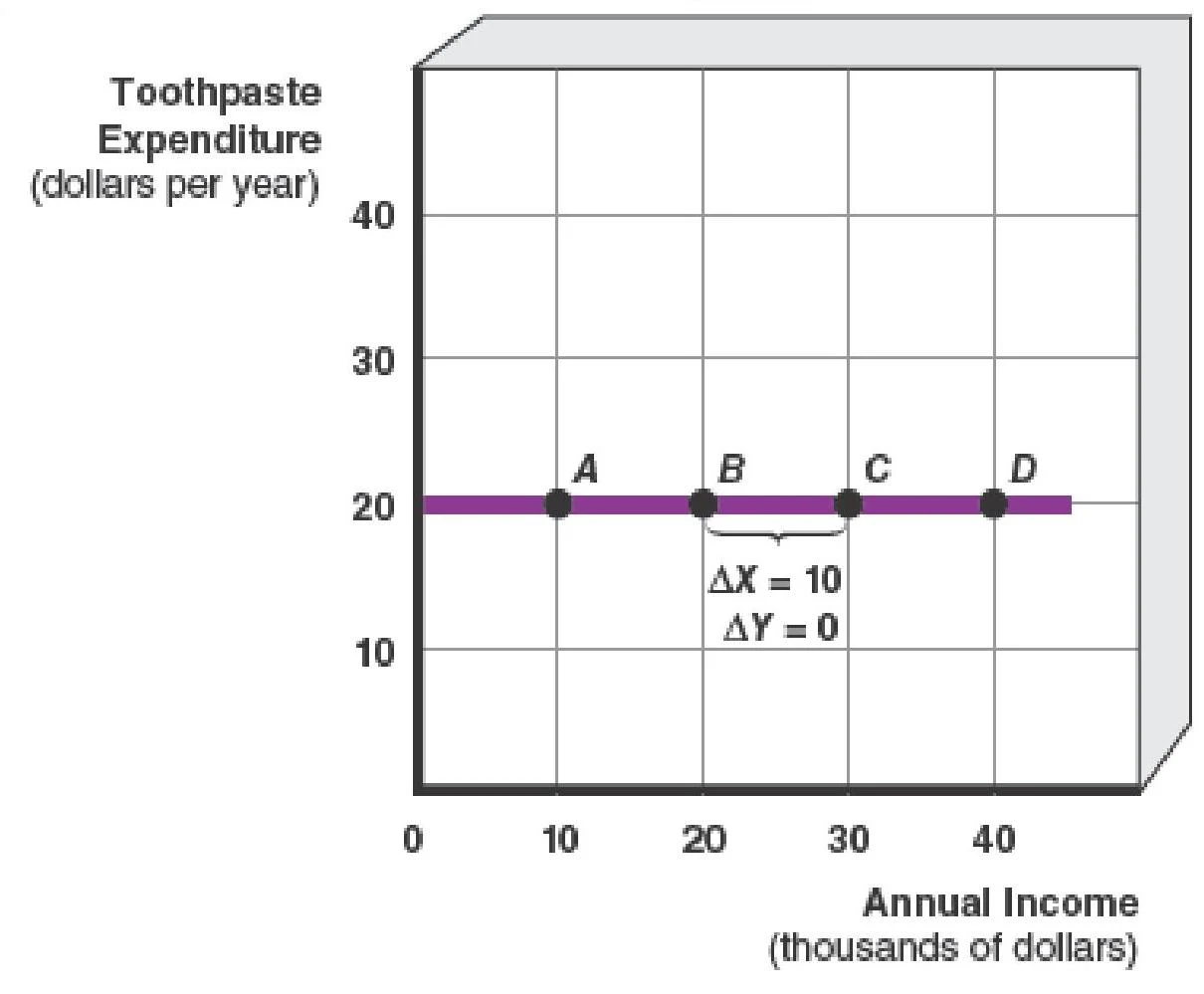
An independent relationship (or zero association) exists when a change in one variable results in no change in the other. Graphically, this is represented by a flat line (either horizontal or vertical). For instance, if consumers spend a constant amount on toothpaste regardless of their annual income, the relationship is independent.
A graph illustrating toothpaste expenditure in dollars per year against annual income in thousands of dollars, showing a constant expenditure regardless of income.
Calculating the Slope
To understand the magnitude of change between variables, economists calculate the slope. The slope is the ratio of the change in the vertical axis variable (the "rise") to the change in the horizontal axis variable (the "run").
Algebraically, if Y is on the vertical axis and X is on the horizontal axis, the slope is:
Slope=runrise=change in horizontal axischange in vertical axis=ΔXΔY
Worked Examples
Example 1: Direct Relationship
Using the PC expenditure data, if income increases from $$20,000to$30,000$ (ΔX=+10) and expenditure increases from $$2,000to$3,000$ (ΔY=+1), the slope is:
Slope=+10+1=0.10
The positive sign indicates an upward-sloping, direct relationship.
Example 2: Inverse Relationship
Using the T-shirt data, if the price decreases by $5 (ΔY=−5) and the quantity purchased increases by 25 million units (ΔX=+25), the slope is:
Slope=+25−5=−51
The negative sign indicates a downward-sloping, inverse relationship.
Study Hint: The steeper a line is, the greater its slope. The flatter the line, the smaller the slope.
Multicurve Graphs: Movements vs. Shifts
In reality, economic models often involve more than two variables. To represent a three-variable relationship on a two-dimensional plane, economists use a multicurve graph.
It is critical to distinguish between a movement along a curve and a shift in a curve:
Movement Along a Curve: This is caused by a change in one of the variables already shown on the coordinate axes. For example, in a price-quantity graph, a change in price causes a movement along the existing demand curve.
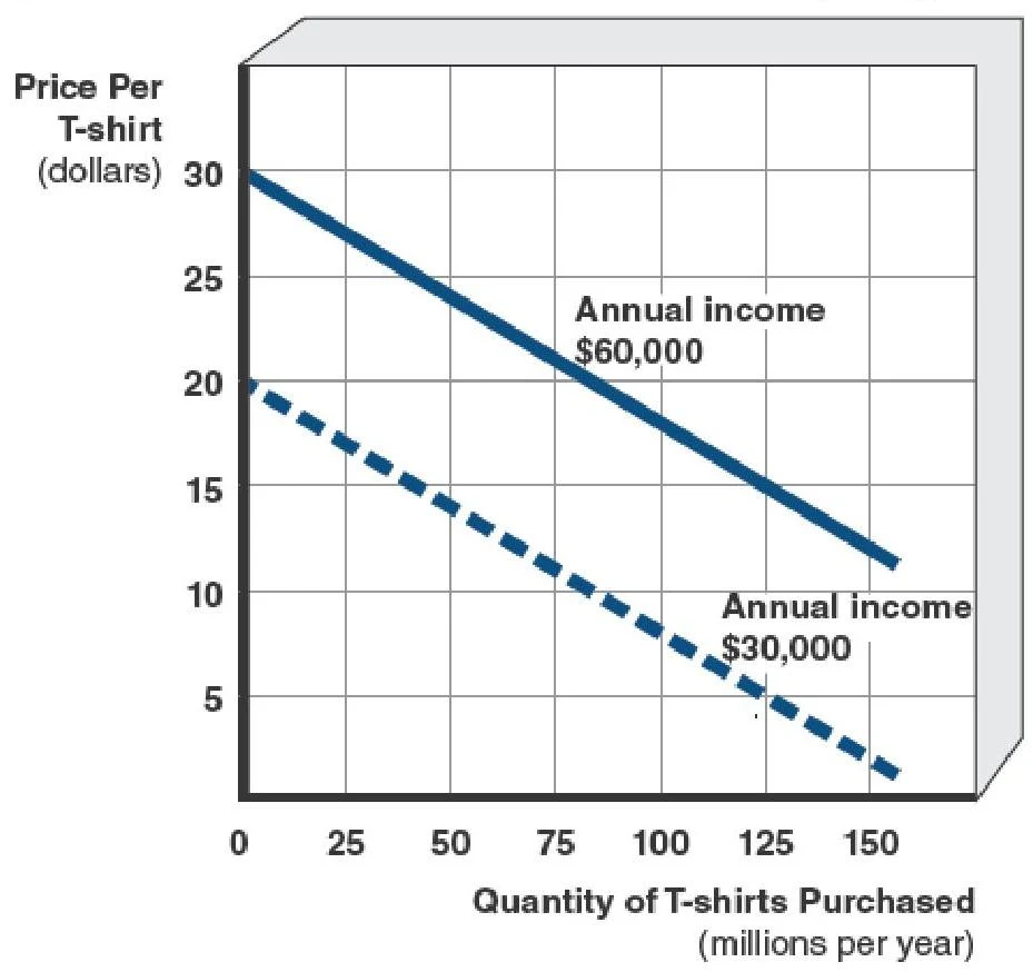
Shift in a Curve: This occurs when a variable not shown on the axes changes, meaning the ceteris paribus assumption has been relaxed. For example, if consumer income increases, the entire demand curve for T-shirts will shift to the right.
This graph illustrates the relationship between the price of t-shirts and the quantity purchased annually by individuals with different annual incomes ($60,000 and $30,000).
Exam Tip: If the variable is on the X or Y axis, it's a movement. If the variable is an "outside" factor (like income or weather), it's a shift.
Keep reading for free.
Create an account to finish this reading and make it part of your study routine.