AP Biology: Experimental Design and Statistical Analysis
Learn the fundamentals of experimental design, including identifying variables, formulating hypotheses, and collecting and visualizing data. This guide covers descriptive statistics like mean and standard deviation, and inferential statistics such as the Chi-square test to determine statistical significance.
In AP Biology, success is not just about knowing the facts of life; it is about understanding how we prove those facts through science. To do this, you must master the language of experimental design and the tools of statistical analysis. Whether you are investigating how temperature affects enzyme activity or how light intensity impacts photosynthesis, you must be able to structure a fair test, visualize your results, and determine if your findings are a biological reality or merely a product of random chance.
Foundations of Experimental Design
A valid experiment is built upon clearly defined variables. If you cannot distinguish between what you change and what you measure, your data will be meaningless.
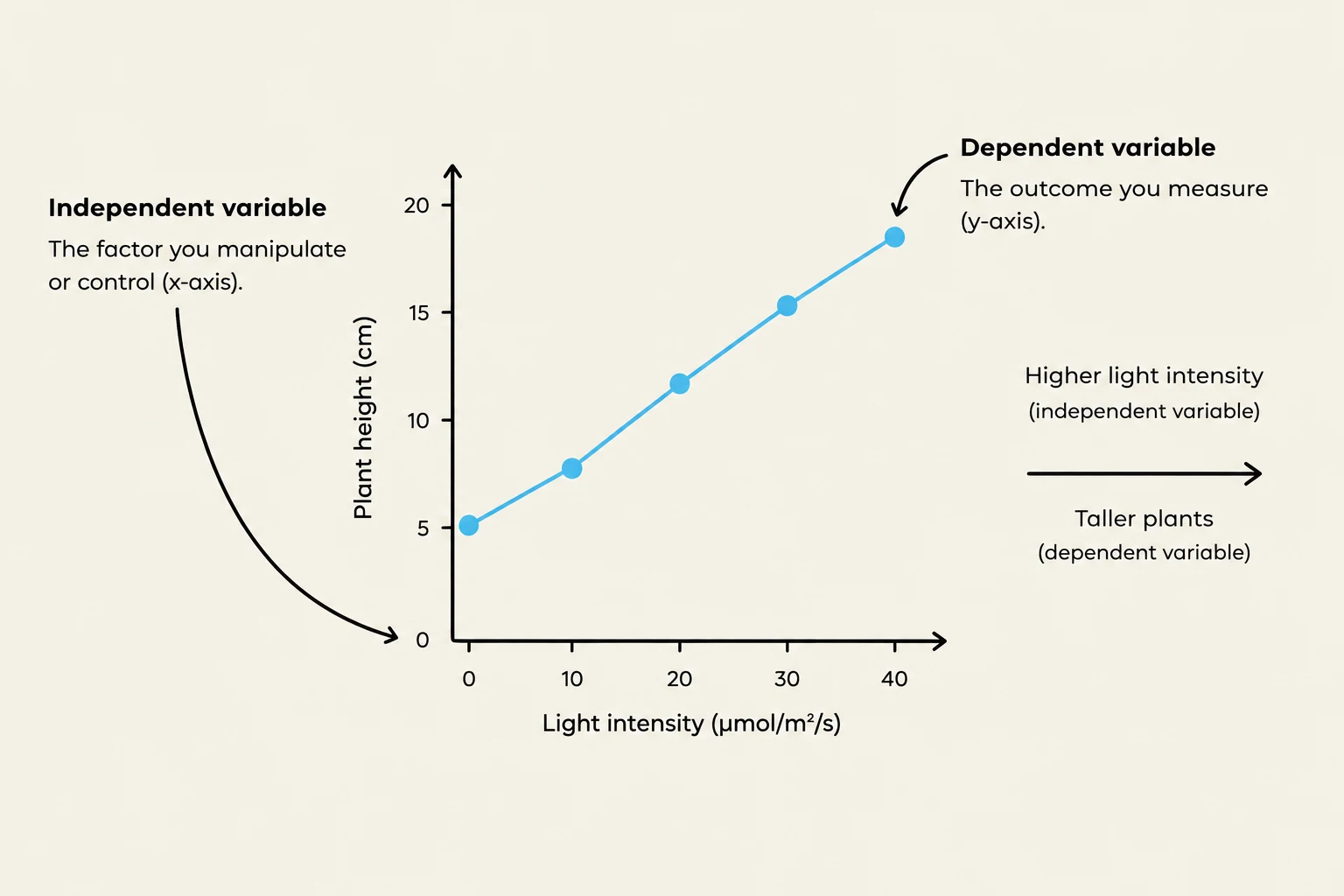
Independent Variable (IV): This is the factor the scientist manipulates or "picks" on purpose. On a graph, the IV is always plotted on the x-axis.
Dependent Variable (DV): This is the responding variable—the thing you measure or "write down" at the end. It is plotted on the y-axis.
Controlled Variables: These are constants kept identical across all groups to ensure a fair test. For example, if testing plant growth, you must keep the soil, pot size, and sunlight the same.
To ensure your results are valid, you must use control groups. A negative control receives no treatment (like plain water) to establish a baseline and show what "no effect" looks like. A positive control receives a known treatment (like a drug known to kill bacteria) to prove that your experimental setup is actually capable of detecting a result.
Exam Tip: The "Effect of" Trick
To avoid swapping your variables, plug them into this sentence: "The effect of [IV] on [DV]." It makes sense to say "The effect of light on plant growth," but it sounds backwards to say "The effect of plant growth on light".
This graph illustrates the relationship between light intensity and plant height, showing that increased light intensity leads to taller plants.
Hypotheses: Experimental vs. Null
A strong experimental hypothesis is a testable, falsifiable statement written in an "If... then... because..." format. It must include the IV, the DV, and a biological rationale.
Conversely, the null hypothesis is the "boring" version used in statistics. It states that there is no significant difference between the observed and expected data, and that any observed difference is due to chance.
Data Collection and Visualization
Data can be quantitative (numerical measurements like 12.5 cm) or qualitative (descriptive qualities like "leaves turned yellow"). To make sense of these numbers, you must choose the correct graph.
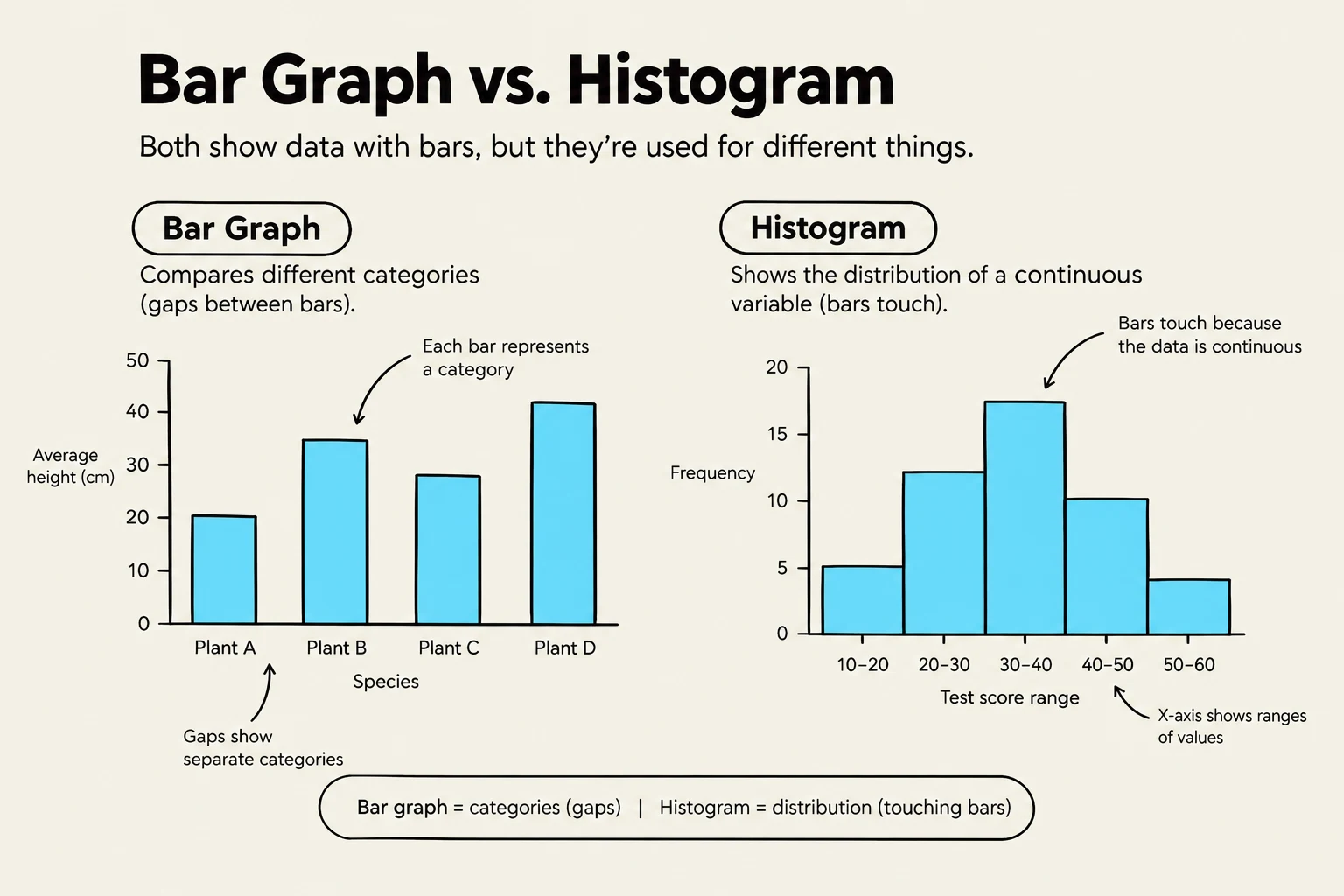
Bar Graphs: Used to compare separate categories (e.g., different species or different fertilizer types). There are gaps between the bars.
Histograms: Used to show the distribution of a single continuous variable (e.g., the heights of 200 sunflowers). Unlike bar graphs, the bars touch.
Line Graphs: Best for showing changes over time or along a continuous scale (e.g., population growth over weeks).
Scatter Plots: Used to show a correlation (relationship) between two numerical variables. You often add a "best-fit line" to show the trend.
Pie Charts: Used to show parts of a whole that total 100%.
When constructing any graph, always use the TAILS checklist: Title (naming both variables), Axes (correct placement), Intervals (even scaling), Labels (including units), and Series key.
This illustration compares bar graphs and histograms, highlighting their distinct uses in data visualization. Bar graphs are used to compare discrete categories, with gaps between bars indicating separate categories. Histograms, on the other hand, display the distribution of continuous data, where bars touch to show the continuity of the variable.
Statistical Analysis: Describing the Data
Once you have collected your data, you need to describe its characteristics using descriptive statistics.
Central Tendency and Spread
Mean (xˉ): The average of the data set.
Median: The middle value when the data is sorted from least to greatest.
Range: The difference between the largest and smallest values.
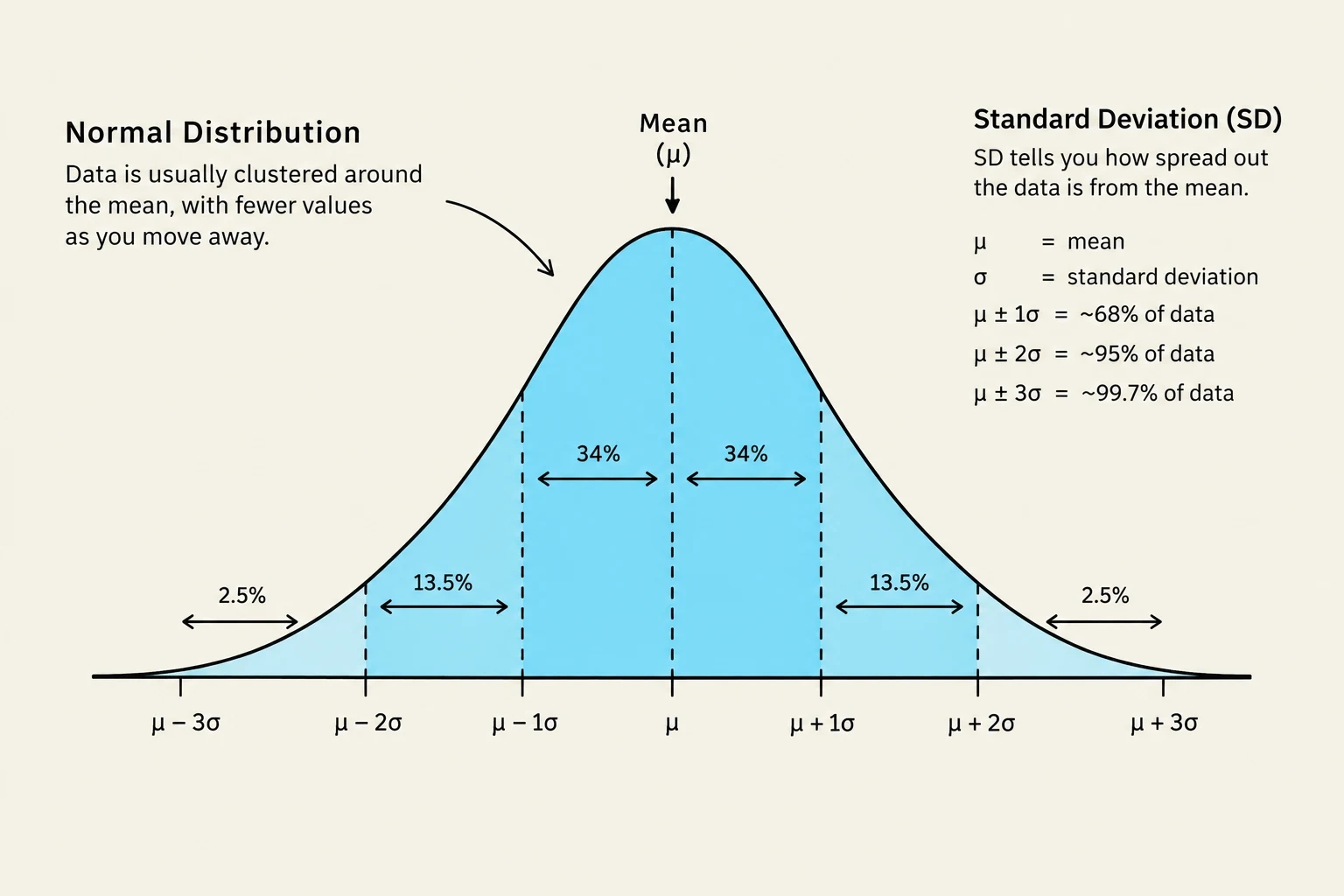
Standard Deviation (SD): This measures how spread out individual data points are around the mean. A large SD indicates high variability, while a small SD indicates data points are clustered closely to the mean. In a normal distribution (a symmetric bell-shaped curve), approximately 68% of data falls within 1 SD of the mean, and 95% falls within 2 SD.
Precision and Reliability
To understand how much we can trust our sample mean, we use the Standard Error of the Mean (SEM). The SEM measures the precision of the sample mean relative to the true population mean. It is calculated as:
SEM=ns
where s is the standard deviation and n is the sample size.
Increasing the sample size (n) is one of the best ways to improve your experiment. A larger n reduces the impact of outliers (extreme, unusual data points), increases reliability (consistency across trials), and decreases the SEM, making your mean more precise.
A normal distribution curve illustrates how data clusters around the mean, with standard deviation indicating the spread of data. Approximately 68% of data falls within one standard deviation, 95% within two, and 99.7% within three.
Determining Statistical Significance
The ultimate goal of AP Bio statistics is to determine statistical significance: is the difference you see real, or is it just luck?
Error Bars
When graphing means, scientists often add error bars representing ±1 SEM.
If error bars overlap, the difference between the means is likely not significant.
If error bars do not overlap, the difference is likely significant.
The Chi-Square (χ2) Test
For categorical data (counts), use the Chi-square test to compare your observed results to your expected results. The formula is:
χ2=∑E(O−E)2
where O is the observed value and E is the expected value.
To interpret the result, you must find the degrees of freedom (df), which is typically (number of categories - 1). You then compare your calculated χ2 to a critical value from a standard table.
If χ2>critical value: Reject the null hypothesis. The difference is significant and not due to chance.
If χ2<critical value: Fail to reject the null hypothesis. The difference is likely due to chance.
Drawing Conclusions
When writing a conclusion, never say you "proved" a hypothesis. Instead, state whether the data supported or refuted it. Use the C-E-R-I method:
Claim: State if the hypothesis was supported.
Evidence: Provide specific numerical data.
Reasoning: Explain the biological mechanism (e.g., "enzyme denaturation occurs at high temperatures").
Improve: Suggest ways to reduce error or future experiments.
Keep reading for free.
Create an account to finish this reading and make it part of your study routine.