Analysis of Nonlinear Systems using Phase Plane and Describing Function Methods

Mathematical Formulation

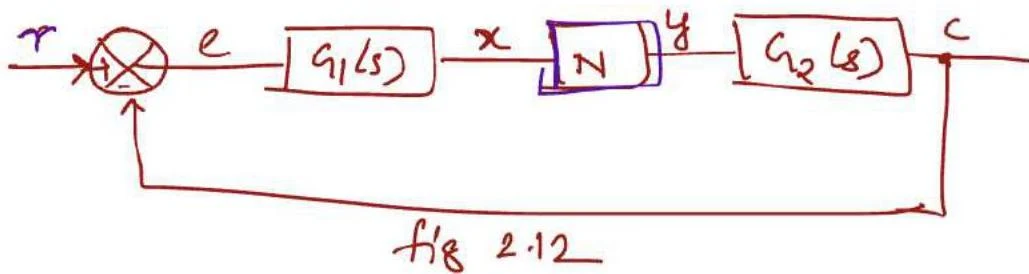
Consider a nonlinear system where the input to the nonlinear element $N$ is a sinusoid $x = X \sin \omega t$. The output $y$ of this nonlinear element is generally a non-sinusoidal periodic function. Using a Fourier series, we can represent this output as a sum of various harmonic components:

$$y = \frac{A_{0} + A_{1} \sin \omega t + B_{1} \cos \omega t + A_{2} \sin 2\omega t + B_{2} \cos 2\omega t + \dots}{1}$$

Because of the low-pass filtering effect mentioned earlier, we focus only on the fundamental component:

$$y_1 = A_1 \sin \omega t + B_1 \cos \omega t = \gamma_1 \sin(\omega t + \phi_1)$$

To find the coefficients of this fundamental component, we use the following integrals:

$$A_1 = \frac{2}{\pi} \int_{0}^{\pi} y \sin \omega t \, d(\omega t)$$ $$B_1 = \frac{2}{\pi} \int_{0}^{\pi} y \cos \omega t \, d(\omega t)$$

From these, we calculate the fundamental amplitude ($\gamma_1$) and the fundamental phase shift ($\phi_1$):

$$\gamma_1 = \sqrt{A_1^2 + B_1^2}$$ $$\phi_1 = \tan^{-1} \frac{B_1}{A_1}$$

The describing function, denoted as $k_N(x, \omega)$, represents the nonlinear element by relating the input amplitude $x$ to the output fundamental amplitude and phase:

$$k_N(x, \omega) = \frac{\gamma_1}{x} \angle \phi_1$$

By replacing the nonlinear block with its describing function, as shown in Figure 2.13, engineers can apply standard linear frequency-domain techniques for stability analysis.

Exam Tip: Remember that the describing function is used for stability analysis, not for direct system design optimization. There is no general correlation between time and frequency responses in nonlinear systems.

Common Nonlinearities

Engineers frequently encounter specific types of nonlinearities that can be analyzed using the describing function method.

1. Relay Nonlinearity

A relay is a common nonlinearity where the output switches between two fixed levels. For a relay with magnitude $m$, the describing function is derived as:

$$k_N(x, \omega) = \frac{4m}{\pi x} \angle -\pi$$

(Note: The phase shift is typically $-\pi$ or $180^\circ$ for a standard relay).

2. Dead Zone Nonlinearity

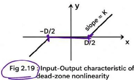
In a dead zone, the output remains zero until the input exceeds a certain threshold ($D/2$).

The describing function for a dead zone is given by:

$$k_N(x, \omega) = k \left[ 1 - \frac{2}{\pi} \left( \sin^{-1} \frac{D}{2x} + \frac{D}{2x} \sqrt{1 - \left(\frac{D}{2x}\right)^2} \right) \right] \angle 0^\circ$$

3. Saturation Nonlinearity

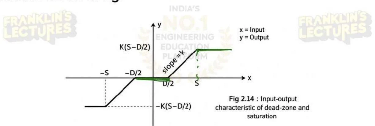
Saturation occurs when the output reaches a maximum limit ($S$) even if the input continues to increase.

The describing function for saturation is:

$$k_N(x, \omega) = \frac{2k}{\pi} \left[ \sin^{-1} \left(\frac{S}{x}\right) + \frac{S}{x} - \sqrt{1 - \left(\frac{S}{x}\right)^2} \right] \angle 0^\circ$$

Summary Comparison