An explanation of the Aggregate Demand (AD) and Aggregate Supply (AS) model in macroeconomics, including the components of AD, factors affecting AD and AS, and market equilibrium.
In macroeconomics, we study the economy as a whole rather than focusing on individual markets. To understand how an entire nation's economy functions, we use the Aggregate Demand (AD) and Aggregate Supply (AS) model. This framework allows economists to analyze how changes in spending and production affect the general price level and the total real output (Real GDP) of a country.
Aggregate Demand (AD)
Aggregate demand represents the total expenditure on goods and services within an economy. Unlike microeconomic demand, which looks at the quantity demanded of a single product, aggregate demand considers the changes in the general price level of all products simultaneously.
The total demand is calculated using the fundamental macroeconomic formula:
AD=C+I+G+(X−M)
where:
Consumption (C): Household spending on goods and services.
Investment (I): Private sector spending on capital goods.
Government Spending (G): Government expenditure on goods and services.
Net Exports (X – M): The difference between the value of exports (X) and imports (M).
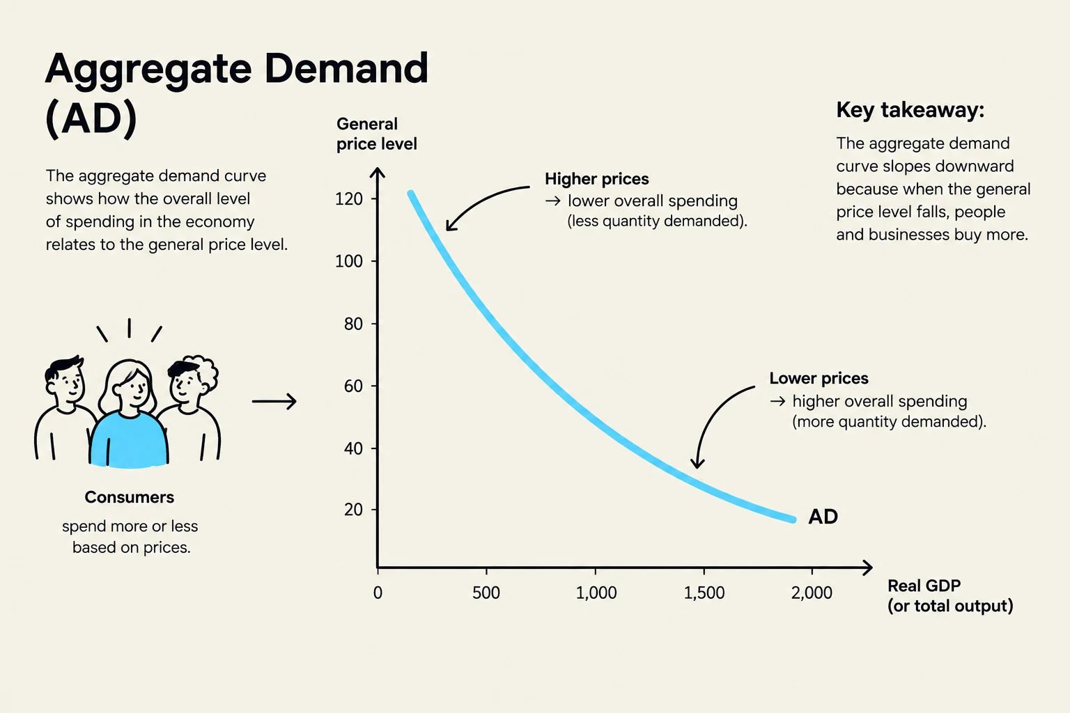
The aggregate demand curve illustrates the relationship between the general price level and the total spending in an economy, showing that as prices fall, overall spending and quantity demanded increase.
Why does the AD curve slope downwards?
The AD curve is downward sloping, meaning a rise in the price level leads to a contraction in aggregate demand, while a fall in the price level leads to an extension in demand. This occurs due to three primary effects:
The Wealth Effect: As the price level rises, the purchasing power of people's wealth (such as savings in bank accounts) falls. This reduction in real wealth leads to lower consumption.
The International Effect: A higher domestic price level makes a country's exports less price-competitive abroad, while making imports relatively cheaper. This causes net exports (X−M) to decrease.
The Interest Rate Effect: A rise in the price level increases the demand for money to cover higher transactions. This increased demand for money drives up interest rates, which in turn reduces both consumption (C) and investment (I).
Shifters of Aggregate Demand
While a change in the price level causes a movement along the AD curve, changes in the non-price components of AD cause the entire curve to shift.
Shifts to the right (Increase in AD): Caused by rising consumer or business confidence, cuts in income or corporation taxes, an increase in the money supply, or a fall in the exchange rate (which boosts exports).
Shifts to the left (Decrease in AD): Caused by factors such as a rise in import values or a decrease in government spending.
Aggregate Supply (AS)
Aggregate supply is the total output (real GDP) that producers in an economy are willing and able to supply at a given price level. Economists distinguish between the short run and the long run because the ability of prices to adjust differs over time.
Short-Run Aggregate Supply (SRAS)
The SRAS curve slopes upward from left to right. This means that as the price level rises, producers are willing to supply more output. This positive relationship exists for three reasons:
The Profit Effect: In the short run, the prices of factors of production (like wages) are often fixed. As the price level rises, the gap between the price of output and the cost of inputs widens, increasing profit margins.
The Cost Effect: To increase output, firms may face rising marginal costs, such as overtime pay or recruitment costs. Producers require higher prices to cover these additional costs.
The Misinterpretation Effect: Producers may confuse an increase in the general price level with an increase in the relative price of their specific product, leading them to believe their product is more popular and thus producing more.
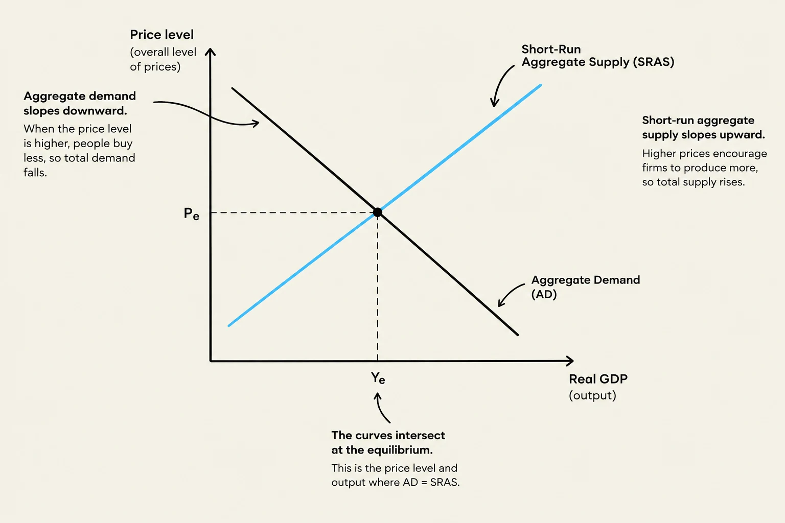
This graph illustrates the aggregate demand and short-run aggregate supply curves, showing their intersection at the equilibrium price level and output.
Shifters of SRAS: The SRAS curve shifts due to changes in the costs of production, such as changes in wage rates, raw material costs, or taxes on firms. Conversely, improvements in factor productivity or technology will shift the SRAS to the right.
Long-Run Aggregate Supply (LRAS)
The LRAS represents the total output an economy can produce when it is using all its factors of production at full employment. There are two major economic perspectives on the shape of the LRAS:
Classical View: Classical economists view the LRAS as a vertical line. They believe the economy naturally operates at full capacity in the long run.
Keynesian View: Keynesian economists argue that the LRAS can have different shapes. It may be perfectly elastic at very low levels of output, upward sloping, and eventually become perfectly inelastic once full capacity is reached. This view emphasizes that economies can operate below full capacity for extended periods.
Exam Tip: Remember that while changes in the price level cause movements along the AS curves, only changes in the quantity or quality of factors of production (FOP) will shift the LRAS curve.
Shifting the LRAS: An increase in the productive potential of an economy (shifting LRAS to the right) can be achieved by:
Increasing the Quantity of FOP: Through net immigration, increasing the retirement age, or discovering new natural resources.
Increasing the Quality of FOP: Through improved education and training (human capital) or advances in technology.
Market Equilibrium
Economic equilibrium occurs at the intersection of the AD and AS curves. This intersection determines the equilibrium price level and the equilibrium real output.
Excess Demand: If the price level is below the equilibrium, there is a shortage of goods and services, which puts upward pressure on prices.
Excess Supply: If the price level is above the equilibrium, there is excess supply (growing inventories), which forces firms to cut prices to clear their stock.
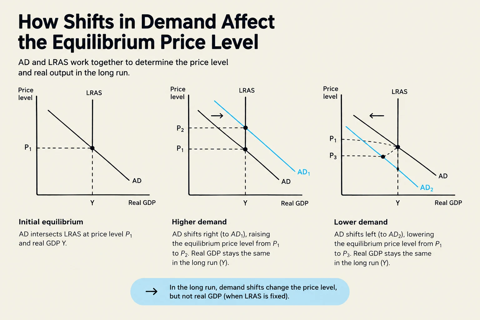
This illustration demonstrates how shifts in aggregate demand (AD) affect the equilibrium price level and real GDP in the long run, assuming the long-run aggregate supply (LRAS) is fixed. It shows an initial equilibrium, followed by scenarios of higher demand leading to increased prices, and lower demand leading to decreased prices, while real GDP remains constant.
Keep reading for free.
Create an account to finish this reading and make it part of your study routine.